Table of contents
- Predicting profitable customer segments
- Proposed steps for solving the tasks
- Dataset investigation
- First approach: try to predict return based on only the first group
- Second approach: try to predict if the campaign should be launched (based on both groups)
- Third approach: try to predict which group should we target
- Fourth approach: try to predict if the campaign should be stopped based on the gX_21 column
- Fifth approach: use additional parameters c_XX to predict the campaign target group
- API for prediction the target group (based of the third approach)
Predicting profitable customer segments
Context
Marketing is a key component of every modern business. Companies continuously re-invest large cuts of their profits for marketing purposes, trying to target groups of customers who have the potential to bring back the highest Return On Investment for the company. The cost of marketing can be very high though, meaning that the decision about which customer group to target is of great financial importance.
This dataset was made available by an online retail company that has collected historical data about such groups of customers, tracked the profitability of each group after the respective marketing campaign, and retrospectively assessed whether investing in marketing spend for that group was a good choice.
Content
To enable machine learning experimentation, this dataset has been structured as follows:
Each row is a comparison between two groups of potential customers:
-
1) Column names starting with “g1” represent characteristics of the first customer group (these were known before the campaign was run)
-
2) Column names starting with “g2” represent characteristics of the second customer group (these were known before the campaign was run)
-
3) Column names starting with “c_” are features representing some comparison of the two groups (also known before the campaign was run)
The last column, named “target” is categorical, with three categories:
- 0 - none of the two groups were profitable
- 1 - group1 turned out to be more profitable
- 2 - group2 turned out to be more profitable
Proposed steps for solving the tasks
5 different approaches were figured out and created for the task:
- First approach: try to predict return based on only the first group.
Basing on the only first group, I have created the model using the DecisionTreeClassifier for prediction of the campaign’s success rate to be launched against this group. Additionally, minmaxscaling and removing of columns g1_XX has been applied in cases where the correlation between them is very high (>0.9). This was used for the reduction of dimensionality.
- Second approach: try to predict if the campaign should be launched (based on both groups).
Basing on both groups, I have created the model using the DecisionTreeClassifier and GradientBoostingClassifier to predict if the campaign should be launched against one of the possible cases (one of the groups, both of them, or simply none). Additionally, minmaxscaling, and removing columns g1_XX have been used for instances where the correlation between them is very high (>0.9) for reduction of dimensionality.
- Third approach: try to predict which group should we target.
Basing on both groups, I have created the model using the GradientBoostingClassifier to predict if the campaign should be launched for the group (one of them, or none of them). Additionally, minmaxscaling and removing columns g1_XX have been used if the correlation between them is very high (>0.9) for reduction of dimensionality in a similar way as two cases before.
- Fourth approach: try to predict if the campaign should be stopped based on the gX_21 column.
Basing on the third approach, an additional step has been added. In this case, another model that tries to catch if the campaign should be stopped is used. The assumption is that the gX_21 features have not been generated in the last stage of the campaign.
- Fifth approach use additional parameters c_XX to predict the campaign target group.
This approach is the connection of the third one and c params. In this case, the c_28 feature is not used (prior is it unknown when the campaign is launched). The created model was made by using the GradientBoostingClassifier to predict if the campaign should be launched for the group (one of them, or none of them)
tl;dr
According to obtained results, it was decided to use the third approach with GradientBoostingClassifier. For this classifier, the accuracy was over 0.54 for the test set. The exported model was used to build an application in python (using the flask library). By using Postman, we can perform queries to select the group for which we want to run marketing activities.
from google.colab import drive
drive.mount('/content/gdrive')
import pandas as pd
import numpy as np
Dataset investigation
Each row is a comparison between two customer groups.
Column names starting with “g1_”:
- contain information about the first customer group
- variables g1_1 until g1_20 were known before the campaign was run
- variable g1_21 was recorded after the campaign was run
Column names starting with “g2_”:
- contain information about the second customer group
- variables g2_1 until g2_20 were known before the campaign was run
- variable g2_21 was recorded after the campaign was run
Column names starting with “c_”:
- contain features representing some comparison of the two groups
- variables c_1 until c_27 were known before the campaign was run
- variable c_28 was recorded after the campaign was run
Target – is categorical. This is what the categories mean:
- 0: none of the two groups were profitable
- 1: group 1 was the most profitable
- 2: group 2 was the most profitable
A caveat: if one of the groups was even slightly better (concerning ROI) then the target we set may affect the result. Based on the dataset, we do not know the return on investment for each group, so we do not know how the results of the two groups differed.
campaign = pd.read_csv('gdrive/My Drive/customer_segments_predicting/customerGroups.csv', sep = ',')
campaign.head()
| g1_1 | g1_2 | g1_3 | g1_4 | g1_5 | g1_6 | g1_7 | g1_8 | g1_9 | g1_10 | g1_11 | g1_12 | g1_13 | g1_14 | g1_15 | g1_16 | g1_17 | g1_18 | g1_19 | g1_20 | g1_21 | g2_1 | g2_2 | g2_3 | g2_4 | g2_5 | g2_6 | g2_7 | g2_8 | g2_9 | g2_10 | g2_11 | g2_12 | g2_13 | g2_14 | g2_15 | g2_16 | g2_17 | g2_18 | g2_19 | g2_20 | g2_21 | c_1 | c_2 | c_3 | c_4 | c_5 | c_6 | c_7 | c_8 | c_9 | c_10 | c_11 | c_12 | c_13 | c_14 | c_15 | c_16 | c_17 | c_18 | c_19 | c_20 | c_21 | c_22 | c_23 | c_24 | c_25 | c_26 | c_27 | c_28 | target | |
|---|---|---|---|---|---|---|---|---|---|---|---|---|---|---|---|---|---|---|---|---|---|---|---|---|---|---|---|---|---|---|---|---|---|---|---|---|---|---|---|---|---|---|---|---|---|---|---|---|---|---|---|---|---|---|---|---|---|---|---|---|---|---|---|---|---|---|---|---|---|---|---|
| 0 | 4.50 | 1 | 3 | 4 | 5 | 1 | 1 | 4 | 6 | 0 | -2 | -2 | 2.505032 | 2.551406 | 6.240000 | 3.608000 | 0.744000 | 1.216000 | 0.003078 | 0.003028 | 0.578205 | 1.83 | 6 | 0 | 6 | 7 | 4 | 0 | 0 | 1 | 4 | -1 | 3 | 2.888736 | 2.616855 | 5.552000 | 0.728000 | 0.160000 | 0.002994 | 0.002953 | 0.586149 | 3.50 | 1.97 | -1 | 7 | 6 | 0 | 0 | 0 | 1 | 3.223605 | 1 | -3 | -2 | 0 | 1 | 4 | 2 | 1 | -6 | -5 | -0.383704 | -0.065449 | 0.584000 | 0.488000 | 0 | -3.232000 | -1.944000 | -0.007944 | 1.76 | 2 |
| 1 | 2.20 | 24 | 22 | 46 | 10 | 24 | 28 | 18 | 22 | -4 | -4 | -8 | 3.718983 | 3.882271 | 7.423435 | 5.048030 | 0.836178 | 1.975244 | 0.784882 | 0.019448 | 0.680013 | 2.80 | 34 | 14 | 48 | 10 | 25 | 16 | 16 | 24 | 9 | -8 | 1 | 4.065822 | 4.042015 | 6.369385 | 1.511704 | 1.783791 | 0.784882 | 0.033373 | 0.498949 | 3.25 | 1.85 | 2 | 1 | 3 | 0 | 0 | 0 | 0 | 1.541039 | 10 | -12 | -2 | 0 | 12 | 2 | -3 | 4 | -13 | -9 | -0.346839 | -0.159744 | -0.947614 | 0.463540 | 0 | -5.342174 | -1.321355 | 0.181064 | 1.85 | 1 |
| 2 | 12.00 | 7 | 4 | 11 | 18 | 8 | 11 | 2 | 10 | -3 | -8 | -11 | 2.244550 | 2.458087 | 11.091399 | 5.853005 | 0.730046 | 2.022004 | 0.043937 | 0.014264 | 0.527707 | 1.30 | 11 | 18 | 29 | 2 | 13 | 3 | 16 | 1 | 10 | 15 | 25 | 4.918483 | 4.050389 | 10.029408 | 2.489174 | 0.204741 | 0.022247 | 0.042004 | 0.567984 | 5.00 | 1.70 | -5 | 10 | 5 | 0 | 0 | 0 | 1 | 2.049024 | -11 | -7 | -18 | 7 | -5 | -1 | -3 | -18 | -18 | -36 | -2.673934 | -1.592303 | 0.525305 | -0.467169 | 0 | -6.566521 | -4.176403 | -0.040277 | 2.05 | 2 |
| 3 | 1.91 | 8 | 5 | 13 | 14 | 6 | 7 | 6 | 9 | -1 | -3 | -4 | 2.580190 | 2.683092 | 9.864426 | 2.582357 | 0.656638 | 1.407549 | 0.041563 | 0.021386 | 0.261785 | 4.50 | 5 | 3 | 8 | 17 | 5 | 9 | 7 | 16 | -4 | -9 | -13 | 1.964163 | 2.278147 | 3.369489 | 0.665585 | 2.163561 | 0.043937 | 0.010358 | 0.273886 | 3.60 | 1.98 | -1 | 3 | 2 | 0 | 0 | 0 | 0 | 2.284503 | 5 | 0 | 5 | -10 | 0 | -3 | 4 | 8 | 1 | 9 | 0.616027 | 0.404945 | -1.506923 | 0.741964 | 0 | -2.438120 | -0.787132 | -0.012101 | 1.82 | 0 |
| 4 | 2.50 | 23 | 16 | 39 | 14 | 33 | 25 | 18 | 27 | 8 | -9 | -1 | 3.470617 | 3.055989 | 11.672962 | 4.554560 | 1.895740 | 1.237122 | 0.941241 | 0.000062 | 0.390180 | 3.00 | 29 | 23 | 52 | 8 | 31 | 22 | 21 | 23 | 9 | -2 | 7 | 4.527831 | 4.215284 | 4.494986 | 1.419174 | 1.144728 | 0.364776 | 0.008148 | 0.347568 | 3.40 | 1.80 | -3 | 2 | -1 | 1 | 0 | 0 | 0 | 2.648418 | 0 | -13 | -13 | 10 | 4 | -4 | -4 | 10 | -18 | -8 | -1.057214 | -1.159294 | 0.751012 | -0.182052 | 0 | -1.259728 | 0.059574 | 0.042613 | 1.99 | 2 |
campaign.describe()
| g1_1 | g1_2 | g1_3 | g1_4 | g1_5 | g1_6 | g1_7 | g1_8 | g1_9 | g1_10 | g1_11 | g1_12 | g1_13 | g1_14 | g1_15 | g1_16 | g1_17 | g1_18 | g1_19 | g1_20 | g1_21 | g2_1 | g2_2 | g2_3 | g2_4 | g2_5 | g2_6 | g2_7 | g2_8 | g2_9 | g2_10 | g2_11 | g2_12 | g2_13 | g2_14 | g2_15 | g2_16 | g2_17 | g2_18 | g2_19 | g2_20 | g2_21 | c_1 | c_2 | c_3 | c_4 | c_5 | c_6 | c_7 | c_8 | c_9 | c_10 | c_11 | c_12 | c_13 | c_14 | c_15 | c_16 | c_17 | c_18 | c_19 | c_20 | c_21 | c_22 | c_23 | c_24 | c_25 | c_26 | c_27 | c_28 | target | |
|---|---|---|---|---|---|---|---|---|---|---|---|---|---|---|---|---|---|---|---|---|---|---|---|---|---|---|---|---|---|---|---|---|---|---|---|---|---|---|---|---|---|---|---|---|---|---|---|---|---|---|---|---|---|---|---|---|---|---|---|---|---|---|---|---|---|---|---|---|---|---|---|
| count | 6620.000000 | 6620.000000 | 6620.000000 | 6620.000000 | 6620.000000 | 6620.000000 | 6620.000000 | 6620.000000 | 6620.000000 | 6620.000000 | 6620.000000 | 6620.000000 | 6620.000000 | 6620.000000 | 6620.000000 | 6620.000000 | 6620.000000 | 6620.000000 | 6620.000000 | 6620.000000 | 6620.000000 | 6620.000000 | 6620.000000 | 6620.000000 | 6620.000000 | 6620.000000 | 6620.000000 | 6620.000000 | 6620.000000 | 6620.000000 | 6620.000000 | 6620.000000 | 6620.000000 | 6620.000000 | 6620.000000 | 6620.000000 | 6620.000000 | 6620.000000 | 6620.000000 | 6620.000000 | 6620.000000 | 6620.000000 | 6620.00000 | 6620.000000 | 6620.000000 | 6620.000000 | 6620.000000 | 6620.000000 | 6620.000000 | 6620.000000 | 6620.000000 | 6620.000000 | 6620.000000 | 6620.000000 | 6620.000000 | 6620.000000 | 6620.000000 | 6620.000000 | 6620.000000 | 6620.000000 | 6620.000000 | 6620.000000 | 6620.000000 | 6620.000000 | 6620.000000 | 6620.00000 | 6620.000000 | 6620.000000 | 6620.000000 | 6620.000000 | 6620.000000 |
| mean | 2.708779 | 14.424018 | 10.485650 | 24.909668 | 10.988066 | 13.412085 | 10.161027 | 10.745468 | 14.169033 | 3.251057 | -3.423565 | -0.172508 | 3.154143 | 3.043544 | 10.268756 | 4.736862 | 1.121263 | 1.159848 | 0.205070 | 0.058852 | 0.449405 | 4.809875 | 15.113897 | 10.018580 | 25.132477 | 11.025076 | 14.040634 | 10.633837 | 10.253323 | 13.500453 | 3.406798 | -3.247130 | 0.159668 | 3.183453 | 3.050268 | 4.840590 | 1.151021 | 1.125410 | 0.205567 | 0.058207 | 0.448996 | 3.899359 | 1.88984 | 1.563595 | 1.558761 | 3.122356 | 0.183686 | 0.200906 | 0.183686 | 0.200906 | 1.945808 | 4.405438 | -4.628248 | -0.222810 | -0.088369 | -0.092296 | 0.111631 | 0.128399 | 6.498187 | -6.830363 | -0.332175 | -0.029311 | -0.006724 | -0.004147 | 0.008827 | 0.00000 | -0.228426 | -0.103728 | 0.000408 | 1.917134 | 1.031722 |
| std | 1.857725 | 10.700787 | 8.384203 | 18.174948 | 5.635985 | 10.090030 | 7.495039 | 7.964247 | 9.866734 | 8.481210 | 8.580752 | 15.036306 | 0.931224 | 0.825628 | 3.760524 | 2.127352 | 0.580622 | 0.566745 | 0.273416 | 0.151767 | 0.139392 | 3.937164 | 10.836923 | 8.251602 | 18.190664 | 5.666965 | 10.205415 | 7.563664 | 7.831935 | 9.722428 | 8.750434 | 8.313375 | 15.025919 | 0.928835 | 0.823931 | 2.150843 | 0.588387 | 0.552912 | 0.273798 | 0.151470 | 0.139194 | 1.093160 | 0.22708 | 4.063520 | 4.057417 | 3.939467 | 0.387257 | 0.400708 | 0.387257 | 0.400708 | 1.217214 | 8.497254 | 9.093944 | 14.470732 | 7.466654 | 6.378463 | 6.343190 | 7.420718 | 12.175872 | 12.973601 | 21.498095 | 1.220752 | 1.068199 | 0.663238 | 0.683422 | 0.32287 | 3.390902 | 1.944419 | 0.092761 | 0.302175 | 0.731042 |
| min | 1.050000 | 0.000000 | 0.000000 | 0.000000 | 1.000000 | 0.000000 | 0.000000 | 0.000000 | 0.000000 | -27.000000 | -38.000000 | -65.000000 | 0.000000 | 0.172875 | 0.000000 | 0.000000 | 0.000000 | 0.000000 | 0.000000 | 0.000000 | 0.000000 | 0.950000 | 0.000000 | 0.000000 | 0.000000 | 1.000000 | 0.000000 | 0.000000 | 0.000000 | 0.000000 | -27.000000 | -36.000000 | -63.000000 | 0.000000 | 0.216094 | 0.000000 | 0.000000 | 0.000000 | 0.000000 | 0.000000 | 0.000000 | 2.500000 | 0.00000 | -10.000000 | -10.000000 | -6.000000 | 0.000000 | 0.000000 | 0.000000 | 0.000000 | 0.000000 | -28.000000 | -47.000000 | -63.000000 | -33.000000 | -29.000000 | -28.000000 | -40.000000 | -39.000000 | -74.000000 | -101.000000 | -4.684111 | -4.319826 | -2.512919 | -3.118836 | -2.00000 | -15.202740 | -9.181722 | -0.750000 | 0.000000 | 0.000000 |
| 25% | 1.667000 | 6.000000 | 4.000000 | 10.000000 | 6.000000 | 5.000000 | 4.000000 | 4.000000 | 6.000000 | -2.000000 | -8.000000 | -8.250000 | 2.499106 | 2.493665 | 8.512643 | 3.389698 | 0.735749 | 0.780218 | 0.011054 | 0.001827 | 0.348935 | 2.500000 | 6.000000 | 3.000000 | 11.000000 | 6.000000 | 6.000000 | 4.000000 | 4.000000 | 5.000000 | -2.000000 | -8.000000 | -8.000000 | 2.500000 | 2.500000 | 3.470612 | 0.760000 | 0.758589 | 0.011054 | 0.001827 | 0.347931 | 3.250000 | 1.74000 | -1.000000 | -1.000000 | 0.000000 | 0.000000 | 0.000000 | 0.000000 | 0.000000 | 0.901358 | 0.000000 | -9.000000 | -7.000000 | -4.000000 | -3.000000 | -3.000000 | -3.000000 | -1.000000 | -13.000000 | -10.000000 | -0.716407 | -0.531224 | -0.440407 | -0.406811 | 0.00000 | -2.222226 | -1.293471 | -0.054331 | 1.710000 | 0.000000 |
| 50% | 2.150000 | 13.000000 | 9.000000 | 22.000000 | 11.000000 | 12.000000 | 9.000000 | 9.000000 | 13.000000 | 1.000000 | -2.000000 | -1.000000 | 2.905237 | 2.764749 | 10.539520 | 4.675946 | 1.079138 | 1.156497 | 0.065102 | 0.006409 | 0.482790 | 3.500000 | 14.000000 | 8.000000 | 22.000000 | 11.000000 | 13.000000 | 10.000000 | 9.000000 | 12.000000 | 1.000000 | -2.000000 | -1.000000 | 2.931093 | 2.769496 | 4.789416 | 1.110897 | 1.126207 | 0.067168 | 0.006314 | 0.483239 | 3.500000 | 1.90000 | 1.000000 | 1.000000 | 2.000000 | 0.000000 | 0.000000 | 0.000000 | 0.000000 | 2.012806 | 3.000000 | -3.000000 | 0.000000 | 0.000000 | 0.000000 | 0.000000 | 0.000000 | 4.000000 | -4.000000 | 0.000000 | 0.000000 | 0.000000 | 0.000000 | 0.001070 | 0.00000 | -0.119378 | -0.012487 | 0.000000 | 1.850000 | 1.000000 |
| 75% | 2.800000 | 21.000000 | 15.000000 | 36.000000 | 16.000000 | 20.000000 | 15.000000 | 16.000000 | 21.000000 | 7.000000 | 1.000000 | 5.000000 | 3.756311 | 3.491114 | 12.500879 | 6.072358 | 1.472574 | 1.533258 | 0.314664 | 0.029305 | 0.554830 | 5.500000 | 22.000000 | 15.000000 | 36.000000 | 16.000000 | 20.000000 | 16.000000 | 15.000000 | 20.000000 | 7.000000 | 1.000000 | 6.000000 | 3.779267 | 3.497749 | 6.221507 | 1.500404 | 1.482003 | 0.314664 | 0.028546 | 0.553774 | 4.000000 | 2.04000 | 4.000000 | 4.000000 | 6.000000 | 0.000000 | 0.000000 | 0.000000 | 0.000000 | 2.982930 | 9.000000 | 1.000000 | 6.000000 | 3.000000 | 3.000000 | 3.000000 | 4.000000 | 13.000000 | 1.000000 | 10.000000 | 0.654627 | 0.490504 | 0.410915 | 0.450104 | 0.00000 | 1.809334 | 1.035235 | 0.054825 | 2.020000 | 2.000000 |
| max | 23.000000 | 52.000000 | 47.000000 | 94.000000 | 20.000000 | 61.000000 | 43.000000 | 48.000000 | 52.000000 | 48.000000 | 31.000000 | 76.000000 | 5.000000 | 4.994496 | 20.502260 | 12.520989 | 3.721637 | 3.185834 | 1.000000 | 1.000000 | 1.000000 | 41.000000 | 55.000000 | 47.000000 | 97.000000 | 20.000000 | 61.000000 | 43.000000 | 45.000000 | 50.000000 | 47.000000 | 31.000000 | 78.000000 | 5.000000 | 4.995596 | 13.428196 | 3.721637 | 3.197138 | 1.000000 | 1.000000 | 1.000000 | 19.000000 | 2.91000 | 13.000000 | 13.000000 | 18.000000 | 1.000000 | 1.000000 | 1.000000 | 1.000000 | 5.334529 | 41.000000 | 33.000000 | 74.000000 | 38.000000 | 23.000000 | 34.000000 | 36.000000 | 75.000000 | 42.000000 | 108.000000 | 4.821136 | 4.396281 | 2.987136 | 2.830550 | 2.00000 | 12.562698 | 8.209578 | 0.666667 | 4.330000 | 2.000000 |
Based on the describe function results, it may be thought that the values in column g2_21 should be scaled as it is in the column g1_21.
# Check the number of nans in df
sum(campaign.isna().sum())
0
campaign[['target']].value_counts()
target
1         3076
2         1877
0         1667
dtype: int64
What percentage of campaigns led to group 1 is the most profitable? What about group 2? And neither of the groups?
Based on the results, more profits generate group 1. In 46.46% the campaign target group 1 gives us good ROI.
campaign[['target']].value_counts()[1]/campaign[['target']].value_counts().sum()*100
target
1         46.465257
dtype: float64
First approach: try to predict return based on only the first group
Basing on the only first group, I have created the model using the DecisionTreeClassifier for prediction of the campaign’s success rate to be launched against this group. Additionally, minmaxscaling and removing of columns g1_XX has been applied in cases where the correlation between them is very high (>0.9). This was used for the reduction of dimensionality.
# Get one hot encoding of columns target to use categorical label in prediction
# The prediction is to get the successful campaign of the first group
one_hot = pd.get_dummies(campaign['target'])

# Join the encoded df
campaign = campaign.join(one_hot)
# Filtering out columns other than group 1, target and encoded target
df_first_group = campaign.filter(regex = 'g1_|target|^[0-9]')
df_first_group
| g1_1 | g1_2 | g1_3 | g1_4 | g1_5 | g1_6 | g1_7 | g1_8 | g1_9 | g1_10 | g1_11 | g1_12 | g1_13 | g1_14 | g1_15 | g1_16 | g1_17 | g1_18 | g1_19 | g1_20 | g1_21 | target | 0 | 1 | 2 | |
|---|---|---|---|---|---|---|---|---|---|---|---|---|---|---|---|---|---|---|---|---|---|---|---|---|---|
| 0 | 4.50 | 1 | 3 | 4 | 5 | 1 | 1 | 4 | 6 | 0 | -2 | -2 | 2.505032 | 2.551406 | 6.240000 | 3.608000 | 0.744000 | 1.216000 | 0.003078 | 0.003028 | 0.578205 | 2 | 0 | 0 | 1 |
| 1 | 2.20 | 24 | 22 | 46 | 10 | 24 | 28 | 18 | 22 | -4 | -4 | -8 | 3.718983 | 3.882271 | 7.423435 | 5.048030 | 0.836178 | 1.975244 | 0.784882 | 0.019448 | 0.680013 | 1 | 0 | 1 | 0 |
| 2 | 12.00 | 7 | 4 | 11 | 18 | 8 | 11 | 2 | 10 | -3 | -8 | -11 | 2.244550 | 2.458087 | 11.091399 | 5.853005 | 0.730046 | 2.022004 | 0.043937 | 0.014264 | 0.527707 | 2 | 0 | 0 | 1 |
| 3 | 1.91 | 8 | 5 | 13 | 14 | 6 | 7 | 6 | 9 | -1 | -3 | -4 | 2.580190 | 2.683092 | 9.864426 | 2.582357 | 0.656638 | 1.407549 | 0.041563 | 0.021386 | 0.261785 | 0 | 1 | 0 | 0 |
| 4 | 2.50 | 23 | 16 | 39 | 14 | 33 | 25 | 18 | 27 | 8 | -9 | -1 | 3.470617 | 3.055989 | 11.672962 | 4.554560 | 1.895740 | 1.237122 | 0.941241 | 0.000062 | 0.390180 | 2 | 0 | 0 | 1 |
| ... | ... | ... | ... | ... | ... | ... | ... | ... | ... | ... | ... | ... | ... | ... | ... | ... | ... | ... | ... | ... | ... | ... | ... | ... | ... |
| 6615 | 1.30 | 3 | 6 | 9 | 1 | 2 | 0 | 9 | 4 | 2 | 5 | 7 | 3.225437 | 2.745887 | 8.128000 | 3.584000 | 1.904000 | 0.728000 | 0.002832 | 0.003089 | 0.440945 | 1 | 0 | 1 | 0 |
| 6616 | 1.85 | 19 | 12 | 31 | 6 | 15 | 9 | 15 | 14 | 6 | 1 | 7 | 3.802635 | 3.643989 | 12.445367 | 3.772041 | 1.275865 | 1.215939 | 0.090605 | 0.064248 | 0.303088 | 0 | 1 | 0 | 0 |
| 6617 | 2.50 | 5 | 8 | 13 | 19 | 3 | 8 | 12 | 10 | -5 | 2 | -3 | 2.639729 | 2.639532 | 12.735732 | 6.930399 | 1.018920 | 1.422971 | 0.056135 | 0.007597 | 0.544170 | 1 | 0 | 1 | 0 |
| 6618 | 1.80 | 5 | 4 | 9 | 10 | 4 | 3 | 2 | 3 | 1 | -1 | 0 | 2.733488 | 2.573255 | 11.668416 | 4.200704 | 0.721472 | 0.597312 | 0.007508 | 0.004967 | 0.360006 | 1 | 0 | 1 | 0 |
| 6619 | 1.95 | 35 | 37 | 72 | 1 | 26 | 15 | 31 | 16 | 11 | 15 | 26 | 5.000000 | 4.931130 | 12.919765 | 4.544010 | 1.411588 | 0.304650 | 0.006134 | 0.923116 | 0.351710 | 0 | 1 | 0 | 0 |
6620 rows × 25 columns
from sklearn.model_selection import train_test_split, cross_val_score

# Exclude g1_21 as the unknown when the campaign is launched
# X is the first group features
X = df_first_group.filter(regex = '^(?!g1_21)g1_')

# y is the successful campaign of the first group
y = df_first_group.loc[:, df_first_group.columns == 1]

# Split the X and our target variable into training and test set
X_train, X_test, y_train, y_test = train_test_split(X, y, test_size = 0.2, random_state = 42)
from sklearn.tree import DecisionTreeClassifier

clf = DecisionTreeClassifier(max_depth = 5, random_state = 0)
clf.fit(X_train, y_train)
cross_val_score(clf, X, y, cv=10)
array([0.66767372, 0.63746224, 0.66616314, 0.63444109, 0.66163142,
       0.65558912, 0.63293051, 0.65558912, 0.64048338, 0.65256798])
from sklearn.metrics import multilabel_confusion_matrix

clf_predictions = clf.predict(X_test)
multilabel_confusion_matrix(y_test, clf_predictions)
array([[[315, 289],
        [169, 551]],

       [[551, 169],
        [289, 315]]])
Of all 1324 test cases, classifier finds 551 launch campaigns that could be categorized as successful and 315 cases that campaign shouldn’t be created. That’s 65.4% accuracy of our classifier.
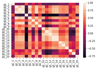
Let’s show the correlation between the encoded target for the first group.
import seaborn as sns
%matplotlib inline

# Calculate the correlation matrix
correlation_train_set = X_train.corr()

# Plot the heatmap to visualise the correlation of the features
sns.heatmap(correlation_train_set,
            xticklabels = correlation_train_set.columns,
            yticklabels = correlation_train_set.columns)
<matplotlib.axes._subplots.AxesSubplot at 0x7fa484318ad0>
# Using preprocessing minmaxscaler to change the range of the feautres
from sklearn import preprocessing

def scale_values(X: pd.DataFrame) -> pd.DataFrame:
  """
  Scale features by minmaxscaler

  """
  x = X.values # Returns a numpy array
  min_max_scaler = preprocessing.MinMaxScaler()
  x_scaled = min_max_scaler.fit_transform(x)
  X_scaled = pd.DataFrame(x_scaled, columns = X.columns)

  return X_scaled

X_train = scale_values(X_train)
Use the correlation between features to get only one column (instead of using all independent variables).
def drop_correlated_features(X_train: pd.DataFrame):
  corr_matrix = X_train.corr().abs()

  # Select upper_part trof correlation matrix
  upper_triangle = corr_matrix.where(np.triu(np.ones(corr_matrix.shape), k=1).astype(np.bool))

  # Find features with correlation greater than 0.90
  features_to_drop = [column for column in upper_triangle.columns if any(upper_triangle[column] > 0.90)]

  # Drop features
  X_train.drop(features_to_drop, axis = 1, inplace=True)

  return X_train, features_to_drop

X_train_scaled, features_to_drop = drop_correlated_features(X_train)
# Save dropped features for further API purposes
import json
with open('/content/gdrive/My Drive/customer_segments_predicting/features_to_drop.json', 'w') as output_json:
    json.dump(features_to_drop, output_json)
# Show selected features
X_train_scaled
| g1_1 | g1_2 | g1_3 | g1_5 | g1_7 | g1_9 | g1_10 | g1_11 | g1_12 | g1_13 | g1_15 | g1_16 | g1_17 | g1_18 | g1_19 | g1_20 | |
|---|---|---|---|---|---|---|---|---|---|---|---|---|---|---|---|---|
| 0 | 0.052392 | 0.096154 | 0.085106 | 0.315789 | 0.023256 | 0.134615 | 0.373333 | 0.478261 | 0.432624 | 0.518286 | 0.378995 | 0.302635 | 0.110128 | 0.357061 | 0.010509 | 0.006738 |
| 1 | 0.006834 | 0.615385 | 0.489362 | 0.105263 | 0.209302 | 0.307692 | 0.613333 | 0.695652 | 0.666667 | 0.987124 | 0.875567 | 0.790637 | 0.456739 | 0.247622 | 0.169272 | 0.522046 |
| 2 | 0.066059 | 0.076923 | 0.021277 | 0.789474 | 0.139535 | 0.096154 | 0.360000 | 0.521739 | 0.446809 | 0.495890 | 0.396688 | 0.355862 | 0.306257 | 0.424941 | 0.008189 | 0.005462 |
| 3 | 0.015945 | 0.134615 | 0.212766 | 0.052632 | 0.046512 | 0.038462 | 0.386667 | 0.608696 | 0.503546 | 0.688240 | 0.589805 | 0.485894 | 0.351539 | 0.178269 | 0.008386 | 0.010620 |
| 4 | 0.093394 | 0.057692 | 0.085106 | 0.736842 | 0.186047 | 0.230769 | 0.293333 | 0.449275 | 0.375887 | 0.410594 | 0.341043 | 0.192402 | 0.188375 | 0.866021 | 0.014462 | 0.007263 |
| ... | ... | ... | ... | ... | ... | ... | ... | ... | ... | ... | ... | ... | ... | ... | ... | ... |
| 5291 | 0.061503 | 0.076923 | 0.063830 | 1.000000 | 0.302326 | 0.307692 | 0.253333 | 0.434783 | 0.347518 | 0.353289 | 0.597160 | 0.578858 | 0.253232 | 0.483775 | 0.088282 | 0.001225 |
| 5292 | 0.030524 | 0.076923 | 0.148936 | 0.578947 | 0.139535 | 0.096154 | 0.306667 | 0.579710 | 0.446809 | 0.545162 | 0.479694 | 0.446075 | 0.303471 | 0.408376 | 0.014462 | 0.006409 |
| 5293 | 0.107062 | 0.192308 | 0.127660 | 1.000000 | 0.674419 | 0.634615 | 0.120000 | 0.231884 | 0.177305 | 0.208641 | 0.510886 | 0.218138 | 0.085544 | 0.797435 | 0.535261 | 0.000003 |
| 5294 | 0.084282 | 0.076923 | 0.212766 | 0.684211 | 0.209302 | 0.038462 | 0.306667 | 0.565217 | 0.439716 | 0.551292 | 0.379544 | 0.219643 | 0.210401 | 0.241557 | 0.025318 | 0.014264 |
| 5295 | 0.027790 | 0.250000 | 0.191489 | 0.263158 | 0.093023 | 0.153846 | 0.480000 | 0.565217 | 0.531915 | 0.728111 | 0.660469 | 0.537986 | 0.374451 | 0.386376 | 0.053598 | 0.030501 |
5296 rows × 16 columns
# Get only selected features based on correlation values
list_of_columns = list(X_train_scaled.columns)

X_selected_features = X[X.columns.intersection(list_of_columns)]
X_selected_features
| g1_1 | g1_2 | g1_3 | g1_5 | g1_7 | g1_9 | g1_10 | g1_11 | g1_12 | g1_13 | g1_15 | g1_16 | g1_17 | g1_18 | g1_19 | g1_20 | |
|---|---|---|---|---|---|---|---|---|---|---|---|---|---|---|---|---|
| 0 | 4.50 | 1 | 3 | 5 | 1 | 6 | 0 | -2 | -2 | 2.505032 | 6.240000 | 3.608000 | 0.744000 | 1.216000 | 0.003078 | 0.003028 |
| 1 | 2.20 | 24 | 22 | 10 | 28 | 22 | -4 | -4 | -8 | 3.718983 | 7.423435 | 5.048030 | 0.836178 | 1.975244 | 0.784882 | 0.019448 |
| 2 | 12.00 | 7 | 4 | 18 | 11 | 10 | -3 | -8 | -11 | 2.244550 | 11.091399 | 5.853005 | 0.730046 | 2.022004 | 0.043937 | 0.014264 |
| 3 | 1.91 | 8 | 5 | 14 | 7 | 9 | -1 | -3 | -4 | 2.580190 | 9.864426 | 2.582357 | 0.656638 | 1.407549 | 0.041563 | 0.021386 |
| 4 | 2.50 | 23 | 16 | 14 | 25 | 27 | 8 | -9 | -1 | 3.470617 | 11.672962 | 4.554560 | 1.895740 | 1.237122 | 0.941241 | 0.000062 |
| ... | ... | ... | ... | ... | ... | ... | ... | ... | ... | ... | ... | ... | ... | ... | ... | ... |
| 6615 | 1.30 | 3 | 6 | 1 | 0 | 4 | 2 | 5 | 7 | 3.225437 | 8.128000 | 3.584000 | 1.904000 | 0.728000 | 0.002832 | 0.003089 |
| 6616 | 1.85 | 19 | 12 | 6 | 9 | 14 | 6 | 1 | 7 | 3.802635 | 12.445367 | 3.772041 | 1.275865 | 1.215939 | 0.090605 | 0.064248 |
| 6617 | 2.50 | 5 | 8 | 19 | 8 | 10 | -5 | 2 | -3 | 2.639729 | 12.735732 | 6.930399 | 1.018920 | 1.422971 | 0.056135 | 0.007597 |
| 6618 | 1.80 | 5 | 4 | 10 | 3 | 3 | 1 | -1 | 0 | 2.733488 | 11.668416 | 4.200704 | 0.721472 | 0.597312 | 0.007508 | 0.004967 |
| 6619 | 1.95 | 35 | 37 | 1 | 15 | 16 | 11 | 15 | 26 | 5.000000 | 12.919765 | 4.544010 | 1.411588 | 0.304650 | 0.006134 | 0.923116 |
6620 rows × 16 columns
# Resample using only selected features
X_train, X_test, y_train, y_test = train_test_split(X_selected_features, y, test_size = 0.2,
                                                    random_state = 42)

clf = DecisionTreeClassifier(max_depth = 5, random_state = 0)
clf.fit(X_train, y_train)
dtree_predictions = clf.predict(X_test)
multilabel_confusion_matrix(y_test, dtree_predictions)
array([[[313, 291],
        [169, 551]],

       [[551, 169],
        [291, 313]]])
Conclusions:
Removing correlated columns gave us much more close results compared to the the original dataframe. This shows than in some cases simplicity of the model allows avoidance of overfitting.
Second approach: try to predict if the campaign should be launched (based on both groups)
Basing on both groups, I have created the model using the GradientBoostingClassifier to predict if the campaign should be launched for the group (one of them, or none of them). Additionally, minmaxscaling and removing columns g1_XX have been used if the correlation between them is very high (>0.9) for reduction of dimensionality in a similar way as two cases before.
# Get first and second group in different df
df_first_group = campaign.filter(regex = '^(?!g1_21)g1_')
df_second_group = campaign.filter(regex = '^(?!g2_21)g2_');
df_second_group.columns = df_first_group.columns

# Append second group to the first one
df_both_groups = df_first_group.append(df_second_group, ignore_index=True)
"""
Get dummy variable as the column of the first group success.
y is the successful campaign of the both group (our target in this approach)
Append second group target (campaign[2]) to the first one (campaign[1])
"""
y = campaign[1]
y = y.append(campaign[2], ignore_index=True)
y.columns = 'y'
df_both_groups['y'] = y
df_both_groups
| g1_1 | g1_2 | g1_3 | g1_4 | g1_5 | g1_6 | g1_7 | g1_8 | g1_9 | g1_10 | g1_11 | g1_12 | g1_13 | g1_14 | g1_15 | g1_16 | g1_17 | g1_18 | g1_19 | g1_20 | y | |
|---|---|---|---|---|---|---|---|---|---|---|---|---|---|---|---|---|---|---|---|---|---|
| 0 | 4.50 | 1 | 3 | 4 | 5 | 1 | 1 | 4 | 6 | 0 | -2 | -2 | 2.505032 | 2.551406 | 6.240000 | 3.608000 | 0.744000 | 1.216000 | 0.003078 | 0.003028 | 0 |
| 1 | 2.20 | 24 | 22 | 46 | 10 | 24 | 28 | 18 | 22 | -4 | -4 | -8 | 3.718983 | 3.882271 | 7.423435 | 5.048030 | 0.836178 | 1.975244 | 0.784882 | 0.019448 | 1 |
| 2 | 12.00 | 7 | 4 | 11 | 18 | 8 | 11 | 2 | 10 | -3 | -8 | -11 | 2.244550 | 2.458087 | 11.091399 | 5.853005 | 0.730046 | 2.022004 | 0.043937 | 0.014264 | 0 |
| 3 | 1.91 | 8 | 5 | 13 | 14 | 6 | 7 | 6 | 9 | -1 | -3 | -4 | 2.580190 | 2.683092 | 9.864426 | 2.582357 | 0.656638 | 1.407549 | 0.041563 | 0.021386 | 0 |
| 4 | 2.50 | 23 | 16 | 39 | 14 | 33 | 25 | 18 | 27 | 8 | -9 | -1 | 3.470617 | 3.055989 | 11.672962 | 4.554560 | 1.895740 | 1.237122 | 0.941241 | 0.000062 | 0 |
| ... | ... | ... | ... | ... | ... | ... | ... | ... | ... | ... | ... | ... | ... | ... | ... | ... | ... | ... | ... | ... | ... |
| 13235 | 12.00 | 6 | 3 | 9 | 3 | 4 | 0 | 2 | 1 | 4 | 1 | 5 | 3.118825 | 2.701205 | 2.912000 | 1.016000 | 0.128000 | 0.002832 | 0.002953 | 0.555725 | 0 |
| 13236 | 4.50 | 9 | 8 | 17 | 16 | 13 | 16 | 5 | 12 | -3 | -7 | -10 | 2.352446 | 2.515035 | 4.177159 | 0.761815 | 1.741461 | 0.197213 | 0.002953 | 0.306024 | 0 |
| 13237 | 2.88 | 6 | 13 | 19 | 7 | 7 | 12 | 12 | 9 | -5 | 3 | -2 | 3.009765 | 2.715531 | 5.770674 | 1.372201 | 1.070904 | 0.051467 | 0.021068 | 0.524975 | 0 |
| 13238 | 5.25 | 2 | 3 | 5 | 15 | 3 | 4 | 3 | 5 | -1 | -2 | -3 | 2.419853 | 2.488684 | 2.804288 | 0.760320 | 1.288640 | 0.008076 | 0.004472 | 0.288826 | 0 |
| 13239 | 4.20 | 28 | 25 | 53 | 6 | 27 | 19 | 27 | 23 | 8 | 4 | 12 | 4.650996 | 4.454084 | 5.036473 | 2.008953 | 1.752584 | 0.199638 | 0.124930 | 0.309187 | 0 |
13240 rows × 21 columns
# Sample train and test chunks
X = df_both_groups.filter(regex = '^g1_')
y = df_both_groups.loc[:, df_both_groups.columns == 'y']
X_train, X_test, y_train, y_test = train_test_split(X, y, test_size = 0.2, random_state = 42)
# Minmaxscale on the train dataset
X_train = scale_values(X_train)
X_train, features_to_drop = drop_correlated_features(X_train)
X_train
| g1_1 | g1_2 | g1_3 | g1_5 | g1_7 | g1_9 | g1_10 | g1_11 | g1_12 | g1_13 | g1_15 | g1_16 | g1_17 | g1_18 | g1_19 | g1_20 | |
|---|---|---|---|---|---|---|---|---|---|---|---|---|---|---|---|---|
| 0 | 0.051186 | 0.200000 | 0.212766 | 0.578947 | 0.232558 | 0.192308 | 0.346667 | 0.536232 | 0.440559 | 0.603098 | 0.321472 | 0.073915 | 0.233640 | 0.038948 | 0.005946 | 0.494133 |
| 1 | 0.051186 | 0.363636 | 0.361702 | 0.631579 | 0.302326 | 0.442308 | 0.413333 | 0.507246 | 0.461538 | 0.702444 | 0.282190 | 0.094862 | 0.411311 | 0.197906 | 0.000187 | 0.509689 |
| 2 | 0.057428 | 0.527273 | 0.382979 | 0.368421 | 0.418605 | 0.461538 | 0.426667 | 0.420290 | 0.426573 | 0.762853 | 0.209630 | 0.082662 | 0.343944 | 0.082729 | 0.013774 | 0.417014 |
| 3 | 0.023720 | 0.290909 | 0.042553 | 0.578947 | 0.279070 | 0.423077 | 0.360000 | 0.376812 | 0.370629 | 0.497270 | 0.460963 | 0.407735 | 0.393238 | 0.529657 | 0.128022 | 0.018316 |
| 4 | 0.035456 | 0.181818 | 0.085106 | 0.473684 | 0.069767 | 0.134615 | 0.413333 | 0.536232 | 0.475524 | 0.631968 | 0.480408 | 0.420553 | 0.398432 | 0.402851 | 0.014114 | 0.008148 |
| ... | ... | ... | ... | ... | ... | ... | ... | ... | ... | ... | ... | ... | ... | ... | ... | ... |
| 10587 | 0.047940 | 0.127273 | 0.021277 | 0.736842 | 0.139535 | 0.096154 | 0.400000 | 0.521739 | 0.461538 | 0.544786 | 0.254946 | 0.117313 | 0.284131 | 0.003487 | 0.005407 | 0.516484 |
| 10588 | 0.019226 | 0.072727 | 0.148936 | 0.578947 | 0.139535 | 0.096154 | 0.306667 | 0.579710 | 0.440559 | 0.545162 | 0.479694 | 0.446075 | 0.303471 | 0.408376 | 0.014462 | 0.006409 |
| 10589 | 0.048689 | 0.072727 | 0.212766 | 0.684211 | 0.209302 | 0.038462 | 0.306667 | 0.565217 | 0.433566 | 0.551292 | 0.379544 | 0.219643 | 0.210401 | 0.241557 | 0.025318 | 0.014264 |
| 10590 | 0.017728 | 0.236364 | 0.191489 | 0.263158 | 0.093023 | 0.153846 | 0.480000 | 0.565217 | 0.524476 | 0.728111 | 0.660469 | 0.537986 | 0.374451 | 0.386376 | 0.053598 | 0.030501 |
| 10591 | 0.300874 | 0.236364 | 0.212766 | 0.894737 | 0.488372 | 0.403846 | 0.280000 | 0.434783 | 0.356643 | 0.470302 | 0.348022 | 0.083209 | 0.386636 | 0.152257 | 0.000747 | 0.572742 |
10592 rows × 16 columns
# Create classifier for the second approach
clf = DecisionTreeClassifier(max_depth = 6, random_state = 0)
clf.fit(X_train, y_train)
DecisionTreeClassifier(ccp_alpha=0.0, class_weight=None, criterion='gini',
                       max_depth=6, max_features=None, max_leaf_nodes=None,
                       min_impurity_decrease=0.0, min_impurity_split=None,
                       min_samples_leaf=1, min_samples_split=2,
                       min_weight_fraction_leaf=0.0, presort='deprecated',
                       random_state=0, splitter='best')
After fitting, let’s rescale using the test dataset with the train set and then dropping the train set
X_scaled = scale_values(X)
# Get only rows with testset
X_test = X_scaled.iloc[X_test.index]
# Drop features
X_test.drop(features_to_drop, axis=1, inplace=True)

clf_predictions = clf.predict(X_test)
multilabel_confusion_matrix(y_test, clf_predictions)
/usr/local/lib/python3.7/dist-packages/pandas/core/frame.py:4174: SettingWithCopyWarning:
A value is trying to be set on a copy of a slice from a DataFrame

See the caveats in the documentation: https://pandas.pydata.org/pandas-docs/stable/user_guide/indexing.html#returning-a-view-versus-a-copy
  errors=errors,


array([[[ 469,  521],
        [ 279, 1379]],

       [[1379,  279],
        [ 521,  469]]])
Accuracy on the combined first and the second group is equal to 69.78%. For 469 cases, the campaign was rightly not released. In contrast, for 1379 occurrences, it was rightly released. For 521 examples, the promotion was not launched even though it would have been profitable, and for 279 cases, the marketing campaign was started even though it should not have been.
from sklearn.model_selection import GridSearchCV
from sklearn.ensemble import GradientBoostingClassifier

# Try another classifier: GradientBoosting with the GridSearchCV to find best params
gbc = GradientBoostingClassifier()
params = {'max_depth':[2, 3, 5, 7],
         'max_leaf_nodes': [3, 4, 5, 6, 7, 8],
         'random_state': [0]}
gs_gbc = GridSearchCV(gbc,
                      param_grid=params,
                      scoring = 'accuracy',
                      cv = 5)
gs_gbc.fit(X_train, y_train.values.ravel())
gs_gbc.score(X_train, y_train)
0.7128965256797583
gs_gbc.best_params_
{'max_depth': 3, 'max_leaf_nodes': 4, 'random_state': 0}
gbc = GradientBoostingClassifier(max_depth = 3, max_features = 'auto',
                                 max_leaf_nodes = 4, random_state = 0)
gbc.fit(X_train, y_train)

X_scaled = scale_values(X)
X_test = X_scaled.iloc[X_test.index]

# Drop features
X_test.drop(features_to_drop, axis = 1, inplace = True)

dtree_predictions = gbc.predict(X_test)
multilabel_confusion_matrix(y_test, dtree_predictions)
/usr/local/lib/python3.7/dist-packages/sklearn/ensemble/_gb.py:1454: DataConversionWarning: A column-vector y was passed when a 1d array was expected. Please change the shape of y to (n_samples, ), for example using ravel().
  y = column_or_1d(y, warn=True)
/usr/local/lib/python3.7/dist-packages/pandas/core/frame.py:4174: SettingWithCopyWarning:
A value is trying to be set on a copy of a slice from a DataFrame

See the caveats in the documentation: https://pandas.pydata.org/pandas-docs/stable/user_guide/indexing.html#returning-a-view-versus-a-copy
  errors=errors,


array([[[ 443,  547],
        [ 217, 1441]],

       [[1441,  217],
        [ 547,  443]]])
Conclusions:
Accuracy agains combined groups is equal to 71.14%. For 443 cases, the campaign shoulnd’t be released. In contrast, for 1441 occurrences, it was released correctly. For 547 examples, the promotion was not launched even though it would have been profitable, and for 217 cases, the marketing campaign was started even though it should not have been.
Third approach: try to predict which group should we target
Basing on both groups, I have created the model using the GradientBoostingClassifier to predict if the campaign should be launched for the group (one of them, or none of them). Additionally, minmaxscaling and removing columns g1_XX have been used if the correlation between them is very high (>0.9) for reduction of dimensionality in a similar way as two cases before.
# X is the first and second group features
df_groups = campaign.filter(regex = '^(?!g1_21)g1_|g2_')
X = df_groups.filter(regex = '^(?!g2_21)')

# y is the successful variable of the first and second group
y = campaign[[1,2]]

X_train, X_test, y_train, y_test = train_test_split(X, y, test_size = 0.2, random_state = 42)
# For the training set get proper groups

def train_set_append_one_group_into_another(X_train: pd.DataFrame):
  """
  To the first group append second group, to store in the same columns as in the first group.
  This is the part for the training set.

  """

  g1_Xtrain = X_train.filter(regex = '^g1_')
  g2_Xtrain = X_train.filter(regex = '^g2_')
  g2_Xtrain.columns = g1_Xtrain.columns

  # To the first group append second group, to store in the same columns as in the first group
  g12_Xtrain = g1_Xtrain.append(g2_Xtrain, ignore_index = True)
  g12_Xtrain_minmax = scale_values(g12_Xtrain)

  # Drop features
  g12_Xtrain_minmax.drop(features_to_drop, axis = 1, inplace = True)
  g12_Xtrain_minmax

  return g12_Xtrain_minmax, g12_Xtrain

g12_Xtrain_minmax, g12_Xtrain = train_set_append_one_group_into_another(X_train)
# Save dropped features for further API purposes
g12_Xtrain.to_json(r'/content/gdrive/My Drive/customer_segments_predicting/g12_Xtrain.json')
# To the first group append second group target, to store in the same columns as in the first group
y = y_train[1].append(y_train[2], ignore_index=True)
gbc = GradientBoostingClassifier(max_depth = 3, max_features = 'auto',
                                 max_leaf_nodes = 4, random_state = 0)
gbc.fit(g12_Xtrain_minmax, y)
GradientBoostingClassifier(ccp_alpha=0.0, criterion='friedman_mse', init=None,
                           learning_rate=0.1, loss='deviance', max_depth=3,
                           max_features='auto', max_leaf_nodes=4,
                           min_impurity_decrease=0.0, min_impurity_split=None,
                           min_samples_leaf=1, min_samples_split=2,
                           min_weight_fraction_leaf=0.0, n_estimators=100,
                           n_iter_no_change=None, presort='deprecated',
                           random_state=0, subsample=1.0, tol=0.0001,
                           validation_fraction=0.1, verbose=0,
                           warm_start=False)
from sklearn.externals import joblib
# Export model to pickle
joblib.dump(clf, '/content/gdrive/My Drive/customer_segments_predicting/model_third.pkl', compress = 1)
/usr/local/lib/python3.7/dist-packages/sklearn/externals/joblib/__init__.py:15: FutureWarning: sklearn.externals.joblib is deprecated in 0.21 and will be removed in 0.23. Please import this functionality directly from joblib, which can be installed with: pip install joblib. If this warning is raised when loading pickled models, you may need to re-serialize those models with scikit-learn 0.21+.
  warnings.warn(msg, category=FutureWarning)


['/content/gdrive/My Drive/customer_segments_predicting/model_third.pkl']
def test_set_append_one_group_into_another(X_test: pd.DataFrame, g12_Xtrain: pd.DataFrame):
  """
  To the first group append second group, to store in the same columns as in the first group.
  This is the part for the test set.

  """
  g1_Xtest = X_test.filter(regex = '^g1_')
  g2_Xtest = X_test.filter(regex = '^g2_')
  g2_Xtest.columns = g1_Xtest.columns
  g12_Xtest = g1_Xtest.append(g2_Xtest, ignore_index = True)

  indexes = g12_Xtest.index.copy()

  # Add training set to make proper minmaxscaling
  g12_Xtest = g12_Xtest.append(g12_Xtrain, ignore_index = True)
  g12_Xtest_minmax = scale_values(g12_Xtest)

  # Drop rows from the training set
  g12_Xtest_minmax = g12_Xtest_minmax.iloc[indexes]

  # Drop features
  g12_Xtest_minmax.drop(features_to_drop, axis = 1, inplace = True)
  g12_Xtest_minmax

  return g12_Xtest_minmax

g12_Xtest_minmax =  test_set_append_one_group_into_another(X_test, g12_Xtrain)
# To the first group append second group target, to store in the same columns as in the first group
y = y_test[1].append(y_test[2], ignore_index = True)

gbc_predictions = gbc.predict(g12_Xtest_minmax)
multilabel_confusion_matrix(y, gbc_predictions)
array([[[ 459,  537],
        [ 230, 1422]],

       [[1422,  230],
        [ 537,  459]]])
prediction_probability = gbc.predict_proba(g12_Xtest_minmax)
prediction_probability = pd.DataFrame(prediction_probability)
Which group to target?
# Get probability from the first group and the second for the same campaign
prediction_probability.iloc[0::int(y.size/2), :]
| 0 | 1 | |
|---|---|---|
| 0 | 0.664091 | 0.335909 |
| 1324 | 0.649775 | 0.350225 |
def dividing_test_set_into_two_groups(prediction_probability: pd.DataFrame, y: pd.DataFrame):
  """
  Dividing the set into two group. As is in the original frame.

  """
  # Divide the appended test set into group 1 and 2

  group_1_prediction_result = prediction_probability.iloc[:int(y.size/2), :]
  group_2_prediction_result = prediction_probability.iloc[int(y.size/2):, :].reset_index()

  group_2_prediction_result.drop('index', axis = 1, inplace = True)
  group_2_prediction_result.columns=['g2_0', 'g2_1']

  joined_results = group_1_prediction_result.join(group_2_prediction_result)

  return joined_results

joined_results = dividing_test_set_into_two_groups(prediction_probability, y)
def prediction_probability_process(prediction_probability: pd.DataFrame,
                                   threshold: float) -> pd.DataFrame:
    """
    Get the target by the comparison of the probability for the first group and
    the second. Additionally, the threshold has been used if the probability
    is low. In this case, none of the target groups should be used for marketing purposes.
    """

    mask = [(prediction_probability[1] >= prediction_probability['g2_1']) &
            (prediction_probability[1] > threshold),
            (prediction_probability[1] < prediction_probability['g2_1']) &
            (prediction_probability['g2_1'] > threshold)]
    prediction_probability['label'] = np.select(mask, [1, 2], default=0)

    return prediction_probability

joined_results = prediction_probability_process(prediction_probability = joined_results,
                                                   threshold = 0.45)
# Get the original label for target
y_target = campaign[['target']]

y_train, y_test = train_test_split(y_target, test_size = 0.2, random_state = 42)
multilabel_confusion_matrix(y_test, joined_results['label'], labels=[0, 1, 2])
array([[[721, 275],
        [190, 138]],

       [[446, 274],
        [179, 425]],

       [[858,  74],
        [254, 138]]])
# Copy the results from this approach, due to usage it in the forth approach
third_approach_y_test = joined_results['label'].copy()
from sklearn.metrics import accuracy_score, precision_score
accuracy_score(y_test, joined_results['label'])
0.5294561933534743
Conclusions:
14 campaigns were not launched in comparison to the original dataset. It has turned out that 13 of these that not launching them was a wrong idea as they gave measurable benefits for both of the groups for each case.
When accuracy is higher than 50%, it means that the created model is more effective than launching campaigns for two groups at the same time. The assumption behind this is that the groups are equal, and thy share same actions costs. Otherwise, it is impossible to compare costs of the campaigns for a given case for both groups.
As it is not known exact moment when the gX_21 index is determined, it is hard to find out of its usefulness in prediction. If it was an indicator calculated shortly after the start of a campaign, it could be used to calculate the correlation with ROI values and used as a stopping marker for campaign run in case of poor results.
Fourth approach: try to predict if the campaign should be stopped based on the gX_21 column
Basing on the third approach, an additional step has been added. In this case, another model that tries to catch if the campaign should be stopped is used. The assumption is that the gX_21 features have not been generated in the last stage of the campaign.
def fourth_approach_train_preprocess(campaign: pd.DataFrame):
    """
    Due to the different scale in the g1_21 and g2_21 columns, the columns
    should be scale separated.

    """
    # X is the first and second group feature (unknown when the campaign start)
    X = campaign.filter(regex = '^g1_21|g2_21')

    # y is the successful variable of the first and second group
    y = campaign[[1, 2]]

    X_train, X_test, y_train, y_test = train_test_split(X, y, test_size = 0.2, random_state = 42)

    # Scale one column, then the second
    g1_Xtrain = X_train.filter(regex = '^g1_')
    g1_Xtrain_minmax = scale_values(g1_Xtrain)
    g1_Xtrain_minmax = pd.DataFrame(g1_Xtrain_minmax)

    g2_Xtrain = X_train.filter(regex = '^g2_')
    g2_Xtrain_minmax = scale_values(g2_Xtrain)
    g2_Xtrain_minmax = pd.DataFrame(g2_Xtrain_minmax).rename(columns={"g2_21": "g1_21"})

    # Append the second group feature into the first one
    g12_Xtrain_minmax = g1_Xtrain_minmax.append(g2_Xtrain_minmax, ignore_index=True)

    y = y_train[1].append(y_train[2], ignore_index=True)

    return X, X_train, X_test, y_train, y_test, g12_Xtrain_minmax, y
def fourth_approach_test_preprocess(X_test: pd.DataFrame,
                                    X: pd.DataFrame):
  """
  Due to the different scale in the g1_21 and g2_21 columns, the columns
  should be scale separated.

  """

  indexes = X_test.index
  #g12_Xtest_minmax = scale_values(X_test)
  g12_Xtest_minmax = scale_values(X)

  # Drop rows from the training set
  g12_Xtest_minmax = g12_Xtest_minmax.iloc[indexes]

  # Append g2_21 into g1_21
  g12_Xtest = g12_Xtest_minmax['g1_21'].append(g12_Xtest_minmax['g2_21'], ignore_index = True)
  g12_Xtest = pd.DataFrame(g12_Xtest, columns = ['g1_21'])

  y = y_test[1].append(y_test[2], ignore_index=True)

  return g12_Xtest, y
GradientBoostingClassifier
# Due to the different scale in the g1_21 and g2_21 columns, the columns should be scale separated.
X, X_train, X_test, y_train, y_test, g12_Xtrain_minmax, y = fourth_approach_train_preprocess(campaign)
g12_Xtrain_minmax
| g1_21 | |
|---|---|
| 0 | 0.487666 |
| 1 | 0.551474 |
| 2 | 0.547860 |
| 3 | 0.503118 |
| 4 | 0.344538 |
| ... | ... |
| 10587 | 0.054545 |
| 10588 | 0.048485 |
| 10589 | 0.042424 |
| 10590 | 0.054545 |
| 10591 | 0.060606 |
10592 rows × 1 columns
gbc = GradientBoostingClassifier(random_state = 0)
gbc.fit(g12_Xtrain_minmax, y)
gbc.score(g12_Xtrain_minmax, y)
0.6549282477341389
g12_Xtest, y = fourth_approach_test_preprocess(X_test, X)

# If the label is zero, then the campaign should be stopped.
gbc_predictions = gbc.predict(g12_Xtest)
multilabel_confusion_matrix(y, gbc_predictions)
array([[[  90,  906],
        [  91, 1561]],

       [[1561,   91],
        [ 906,   90]]])
def prediction_probability_fourth_approach_processing(prediction_probability: pd.DataFrame) -> pd.DataFrame:
    """
    Get the target by the comparison of the probability for the first group and
    the second. Additionally, the threshold has been used if the probability
    is low. In this case, none of the target groups should be used for marketing purposes.
    """
    mask = [(prediction_probability[1] >= prediction_probability['g2_0']), # Don't stop campaign
         (prediction_probability[1] < prediction_probability['g2_0'])]

    prediction_probability['label'] = np.select(mask, [1, 0], default=0)

    return prediction_probability
prediction_probability = gbc.predict_proba(g12_Xtest)
prediction_probability = pd.DataFrame(prediction_probability)

joined_g_21 = dividing_test_set_into_two_groups(prediction_probability, y)
joined_g_21 = prediction_probability_fourth_approach_processing(joined_g_21)
prediction_probability
| 0 | 1 | |
|---|---|---|
| 0 | 0.538459 | 0.461541 |
| 1 | 0.504122 | 0.495878 |
| 2 | 0.524196 | 0.475804 |
| 3 | 0.807927 | 0.192073 |
| 4 | 0.541904 | 0.458096 |
| ... | ... | ... |
| 2643 | 0.671757 | 0.328243 |
| 2644 | 0.661518 | 0.338482 |
| 2645 | 0.701733 | 0.298267 |
| 2646 | 0.701733 | 0.298267 |
| 2647 | 0.701733 | 0.298267 |
2648 rows × 2 columns
# y is the target variable
y = campaign['target']

y_train, y_test = train_test_split(y, test_size = 0.2, random_state = 42)

# Copy to results to use it in further comparison
y_target = y_test.copy()
y_target_original = y_test.copy()

multilabel_confusion_matrix(y_test, joined_g_21['label'], labels=[0, 1])
array([[[  5, 991],
        [  1, 327]],

       [[716,   4],
        [602,   2]]])
def processing_y_target(y_target: pd.DataFrame,
                        third_y_test: pd.DataFrame,
                        joined_g_21: pd.DataFrame) -> pd.DataFrame:
  """
  Get the results from the third and forth approach, to stop campaigns that
  might be unsuccessful. If the campaign is predicted as group 1 or 2, then
  the check is made to the classifier of the gX_21 params.

  """

  y_target_results = pd.DataFrame(y_target.reset_index().drop('index', axis=1))

  y_target_results['third'] = third_y_test
  y_target_results['label'] = joined_g_21['label']

  mask = [((y_target_results['third'] == 1) | (y_target_results['third'] == 2) ) &
          (y_target_results['label'] == 0), # Stop campaign
          (y_target_results['third'] == 1),
          (y_target_results['third'] == 2)]
  y_target_results['label'] = np.select(mask, [0, 1, 2], default=0)

  return y_target_results
joined_g_21 = processing_y_target(y_target=y_target,
                                  third_y_test=third_approach_y_test,
                                  joined_g_21=joined_g_21)
multilabel_confusion_matrix(y_target_original, joined_g_21['label'], labels=[0, 1, 2])
array([[[  4, 992],
        [  1, 327]],

       [[718,   2],
        [602,   2]],

       [[932,   0],
        [391,   1]]])
accuracy_score(y_target_original, joined_g_21['label'])
0.24924471299093656
precision_score(y_target_original, joined_g_21['label'], average='weighted')
0.5855862149527359
LogisticRegression
https://i.pinimg.com/originals/f6/dc/ab/f6dcabbfe346ea36f4a71e60542657bc.jpg
# Trying to get better results by the LogisticRegression
from sklearn.linear_model import LogisticRegression

X, X_train, X_test, y_train, y_test, g12_Xtrain_minmax, y = fourth_approach_train_preprocess(campaign)

logreg = LogisticRegression()
params = {'class_weight': [{ 0:0.5, 1:0.8 }, { 0:0.3, 1:0.8 }, { 0:1.0, 1:0.8 },
                           { 0:1.2, 1:0.8 }, { 0:1.5, 1:0.8 }, { 0:1.8, 1:0.8 },
                           { 0:3, 1:0.8 }],
          'random_state': [0]}

# By using gridsearchcv, try to find best params
gs_logreg = GridSearchCV(logreg,
                      param_grid = params,
                      scoring = 'precision',
                      cv = 5)
gs_logreg.fit(g12_Xtrain_minmax, y)
gs_logreg.score(g12_Xtrain_minmax, y)
0.4730785931393834
gs_logreg.best_params_
{'class_weight': {0: 0.5, 1: 0.8}, 'random_state': 0}
logreg = LogisticRegression(class_weight = {0: 0.5, 1: 0.8}, random_state = 0)
logreg.fit(g12_Xtrain_minmax, y)

g12_Xtest, y = fourth_approach_test_preprocess(X_test, X)

logreg_predictions = logreg.predict(g12_Xtest)
multilabel_confusion_matrix(y, logreg_predictions)
array([[[ 535,  461],
        [ 637, 1015]],

       [[1015,  637],
        [ 461,  535]]])
prediction_probability = logreg.predict_proba(g12_Xtest)
prediction_probability = pd.DataFrame(prediction_probability)

joined_g_21 = dividing_test_set_into_two_groups(prediction_probability, y)
joined_g_21 = prediction_probability_fourth_approach_processing(joined_g_21)

joined_g_21 = processing_y_target(y_target=y_target,
                                  third_y_test=third_approach_y_test,
                                  joined_g_21=joined_g_21)
multilabel_confusion_matrix(y_target_original, joined_g_21['label'], labels=[0, 1, 2])
array([[[238, 758],
        [ 62, 266]],

       [[640,  80],
        [441, 163]],

       [[913,  19],
        [354,  38]]])
accuracy_score(y_target_original, joined_g_21['label'])
0.3527190332326284
precision_score(y_target_original, joined_g_21['label'], average='weighted')
0.5677407263654222
KNN
# Trying to get better results by the KNeighborsClassifier
from sklearn.neighbors import KNeighborsClassifier

X, X_train, X_test, y_train, y_test, g12_Xtrain_minmax, y = fourth_approach_train_preprocess(campaign)

knn = KNeighborsClassifier(20)
knn.fit(g12_Xtrain_minmax, y)
KNeighborsClassifier(algorithm='auto', leaf_size=30, metric='minkowski',
                     metric_params=None, n_jobs=None, n_neighbors=20, p=2,
                     weights='uniform')
g12_Xtest, y = fourth_approach_test_preprocess(X_test, X)

knn_predictions = knn.predict(g12_Xtest)
multilabel_confusion_matrix(y, knn_predictions)
array([[[ 219,  777],
        [ 231, 1421]],

       [[1421,  231],
        [ 777,  219]]])
prediction_probability = knn.predict_proba(g12_Xtest)
prediction_probability = pd.DataFrame(prediction_probability)

joined_g_21 = dividing_test_set_into_two_groups(prediction_probability, y)
joined_g_21 = prediction_probability_fourth_approach_processing(joined_g_21)

joined_g_21 = processing_y_target(y_target=y_target,
                                  third_y_test=third_approach_y_test,
                                  joined_g_21=joined_g_21)

multilabel_confusion_matrix(y_target, third_approach_y_test, labels=[0, 1, 2])
array([[[721, 275],
        [190, 138]],

       [[446, 274],
        [179, 425]],

       [[858,  74],
        [254, 138]]])
accuracy_score(y_target, joined_g_21['label'])
0.2756797583081571
precision_score(y_target, joined_g_21['label'], average='weighted')
0.5467943162033351
Conclusions
For the three classification methods selected, the best obtained accuracy was for logistic regression. Achieved precision is above 0.5. It should be borne in mind that campaign discontinuation is an aggressive operation. With an increased threshold, we obtain more possible exits for campaigns that were misplaced. However, based on further research, it appears that out of 3 closed advertising campaigns, one was rightly closed, and others were not. This method can be used for conducting risk-free campaigns. For example when we minimize the risk of unsuccessful results and do not agree to keep running a campaign that does not have a high level of predicted success.
Fifth approach: use additional parameters c_XX to predict the campaign target group
This approach is the connection of the third one and c params. In this case, the c_28 feature is not used (prior is it unknown when the campaign is launched). The created model was made by using the GradientBoostingClassifier to predict if the campaign should be launched for the group (one of them, or none of them)
Preprocessing c_XX params
# X is the difference between first and second group feature
X = campaign.filter(regex = '^g1_21|g2_21')

# y is the target variable
X = campaign.filter(regex = '^(?!c_28)c_')
y = campaign[['target']]

c_Xtrain, c_Xtest, c_ytrain, c_ytest = train_test_split(X, y, test_size = 0.2, random_state = 42)
# c_ parameters process
c_Xtrain_minmax = scale_values(c_Xtrain)
c_Xtrain_minmax, features_to_drop_c = drop_correlated_features(c_Xtrain_minmax)
c_Xtrain_minmax.describe()
| c_1 | c_2 | c_3 | c_4 | c_5 | c_6 | c_7 | c_8 | c_9 | c_10 | c_11 | c_12 | c_13 | c_14 | c_15 | c_16 | c_22 | c_23 | c_24 | c_25 | c_26 | c_27 | |
|---|---|---|---|---|---|---|---|---|---|---|---|---|---|---|---|---|---|---|---|---|---|---|
| count | 5296.000000 | 5296.000000 | 5296.000000 | 5296.000000 | 5296.000000 | 5296.000000 | 5296.000000 | 5296.000000 | 5296.000000 | 5296.000000 | 5296.000000 | 5296.000000 | 5296.000000 | 5296.000000 | 5296.000000 | 5296.000000 | 5296.000000 | 5296.000000 | 5296.000000 | 5296.000000 | 5296.000000 | 5296.000000 |
| mean | 0.649838 | 0.502660 | 0.501970 | 0.379437 | 0.184479 | 0.201662 | 0.186367 | 0.200906 | 0.366538 | 0.469635 | 0.530020 | 0.450418 | 0.464033 | 0.555183 | 0.453239 | 0.527277 | 0.476340 | 0.525231 | 0.500661 | 0.540350 | 0.514888 | 0.529449 |
| std | 0.078580 | 0.175948 | 0.174259 | 0.162854 | 0.387911 | 0.401279 | 0.389439 | 0.400716 | 0.227989 | 0.122383 | 0.113747 | 0.107156 | 0.105564 | 0.123941 | 0.101785 | 0.098069 | 0.125665 | 0.115529 | 0.082022 | 0.122678 | 0.114175 | 0.066214 |
| min | 0.000000 | 0.000000 | 0.000000 | 0.000000 | 0.000000 | 0.000000 | 0.000000 | 0.000000 | 0.000000 | 0.000000 | 0.000000 | 0.000000 | 0.000000 | 0.000000 | 0.000000 | 0.000000 | 0.000000 | 0.000000 | 0.000000 | 0.000000 | 0.000000 | 0.000000 |
| 25% | 0.601375 | 0.391304 | 0.391304 | 0.250000 | 0.000000 | 0.000000 | 0.000000 | 0.000000 | 0.170619 | 0.405797 | 0.475000 | 0.400000 | 0.408451 | 0.500000 | 0.403226 | 0.486842 | 0.394525 | 0.455303 | 0.500000 | 0.468022 | 0.444111 | 0.490484 |
| 50% | 0.652921 | 0.478261 | 0.478261 | 0.333333 | 0.000000 | 0.000000 | 0.000000 | 0.000000 | 0.377950 | 0.449275 | 0.550000 | 0.451852 | 0.464789 | 0.557692 | 0.451613 | 0.526316 | 0.477129 | 0.524228 | 0.500000 | 0.544114 | 0.519365 | 0.529412 |
| 75% | 0.701031 | 0.608696 | 0.608696 | 0.458333 | 0.000000 | 0.000000 | 0.000000 | 0.000000 | 0.562930 | 0.536232 | 0.600000 | 0.496296 | 0.507042 | 0.615385 | 0.500000 | 0.578947 | 0.554696 | 0.598987 | 0.500000 | 0.614504 | 0.580805 | 0.568348 |
| max | 1.000000 | 1.000000 | 1.000000 | 1.000000 | 1.000000 | 1.000000 | 1.000000 | 1.000000 | 1.000000 | 1.000000 | 1.000000 | 1.000000 | 1.000000 | 1.000000 | 1.000000 | 1.000000 | 1.000000 | 1.000000 | 1.000000 | 1.000000 | 1.000000 | 1.000000 |
# For the test set process to drop redundant columns
indexes = c_Xtest.index

# Add training set to the test, to make better scaling
c_test = c_Xtest.append(c_Xtrain, ignore_index = True)
c_Xtest_minmax = scale_values(c_test)

# Drop rows from the training set
c_Xtest_minmax = c_Xtest_minmax.iloc[indexes]

# Drop features
c_Xtest_minmax.drop(features_to_drop_c, axis = 1, inplace = True)
c_Xtest_minmax
| c_1 | c_2 | c_3 | c_4 | c_5 | c_6 | c_7 | c_8 | c_9 | c_10 | c_11 | c_12 | c_13 | c_14 | c_15 | c_16 | c_22 | c_23 | c_24 | c_25 | c_26 | c_27 | |
|---|---|---|---|---|---|---|---|---|---|---|---|---|---|---|---|---|---|---|---|---|---|---|
| 96 | 0.670103 | 0.608696 | 0.434783 | 0.416667 | 0.0 | 0.0 | 0.0 | 0.0 | 0.598998 | 0.623188 | 0.5500 | 0.547445 | 0.408451 | 0.576923 | 0.258065 | 0.605263 | 0.215120 | 0.608343 | 0.5 | 0.609119 | 0.574976 | 0.525365 |
| 994 | 0.604811 | 0.434783 | 0.782609 | 0.583333 | 0.0 | 1.0 | 0.0 | 0.0 | 0.531604 | 0.391304 | 0.5875 | 0.452555 | 0.549296 | 0.480769 | 0.661290 | 0.355263 | 0.711773 | 0.291270 | 0.5 | 0.665812 | 0.525615 | 0.473125 |
| 1400 | 0.649485 | 0.521739 | 0.434783 | 0.333333 | 0.0 | 0.0 | 0.0 | 0.0 | 0.607934 | 0.405797 | 0.5875 | 0.459854 | 0.464789 | 0.557692 | 0.451613 | 0.526316 | 0.456890 | 0.524228 | 0.5 | 0.547542 | 0.527949 | 0.529412 |
| 865 | 0.608247 | 0.695652 | 0.391304 | 0.458333 | 1.0 | 0.0 | 0.0 | 0.0 | 0.023845 | 0.478261 | 0.6250 | 0.518248 | 0.507042 | 0.576923 | 0.419355 | 0.486842 | 0.453445 | 0.499239 | 0.5 | 0.752380 | 0.696666 | 0.621067 |
| 6095 | 0.707904 | 0.478261 | 0.434783 | 0.291667 | 0.0 | 0.0 | 0.0 | 0.0 | 0.460720 | 0.492754 | 0.6250 | 0.525547 | 0.436620 | 0.634615 | 0.387097 | 0.539474 | 0.423508 | 0.544828 | 0.5 | 0.343235 | 0.340730 | 0.500116 |
| ... | ... | ... | ... | ... | ... | ... | ... | ... | ... | ... | ... | ... | ... | ... | ... | ... | ... | ... | ... | ... | ... | ... |
| 4706 | 0.707904 | 0.478261 | 0.652174 | 0.500000 | 0.0 | 0.0 | 0.0 | 0.0 | 0.464967 | 0.405797 | 0.5625 | 0.445255 | 0.366197 | 0.615385 | 0.596774 | 0.605263 | 0.601209 | 0.543221 | 0.5 | 0.637394 | 0.574294 | 0.485308 |
| 1272 | 0.680412 | 0.565217 | 0.869565 | 0.791667 | 1.0 | 1.0 | 0.0 | 0.0 | 0.142904 | 0.565217 | 0.5875 | 0.540146 | 0.760563 | 0.442308 | 0.725806 | 0.500000 | 0.639388 | 0.412323 | 0.5 | 0.516780 | 0.544211 | 0.559017 |
| 6309 | 0.676976 | 0.869565 | 0.347826 | 0.583333 | 1.0 | 1.0 | 1.0 | 0.0 | 0.567412 | 0.420290 | 0.6500 | 0.503650 | 0.450704 | 0.326923 | 0.451613 | 0.486842 | 0.399996 | 0.414049 | 1.0 | 0.409835 | 0.463331 | 0.539959 |
| 4479 | 0.477663 | 0.565217 | 0.304348 | 0.250000 | 1.0 | 1.0 | 0.0 | 0.0 | 0.532125 | 0.782609 | 0.8625 | 0.810219 | 0.619718 | 0.538462 | 0.629032 | 0.434211 | 0.566057 | 0.351052 | 0.5 | 0.629507 | 0.669657 | 0.581510 |
| 6037 | 0.615120 | 0.869565 | 0.478261 | 0.708333 | 0.0 | 0.0 | 0.0 | 1.0 | 0.543473 | 0.536232 | 0.4375 | 0.437956 | 0.718310 | 0.250000 | 0.580645 | 0.328947 | 0.580161 | 0.479086 | 0.5 | 0.588110 | 0.493371 | 0.483194 |
1324 rows × 22 columns
Processing params g1 and g2
df_groups = campaign.filter(regex = '^(?!g1_21)g1_|g2_')

# X is the first and second group features
X = df_groups.filter(regex = '^(?!g2_21)')

# y is the target variable
y = campaign['target']

X_train, X_test, y_train, y_test = train_test_split(X, y, test_size = 0.2, random_state = 42)

# For the training set get proper groups as the one of the column in the dataframe
# to use it in modeling as the one of the feature
g1_Xtrain = X_train.filter(regex = '^g1_')
g1_Xtrain['group'] = 1
g2_Xtrain = X_train.filter(regex = '^g2_')
g2_Xtrain['group'] = 2
g2_Xtrain.columns = g1_Xtrain.columns
g12_Xtrain = g1_Xtrain.append(g2_Xtrain, ignore_index = True)

# Scale the value other for other than group column
g12_Xtrain_without_groups = g12_Xtrain.loc[:, g12_Xtrain.columns != 'group']
g12_Xtrain_without_groups_minmax = scale_values(g12_Xtrain_without_groups)

# Drop features by the correlation as in the previous approaches
g12_Xtrain_without_groups_minmax.drop(features_to_drop, axis = 1, inplace = True)
g12_Xtrain_without_groups_minmax['group'] = g12_Xtrain['group']

c_Xtest_minmax_appended = c_Xtrain_minmax.append(c_Xtrain_minmax, ignore_index = True)
y_train_appended=y_train.append(y_train, ignore_index = True)

result = pd.concat([g12_Xtrain_without_groups_minmax, c_Xtest_minmax_appended], axis = 1)
result
/usr/local/lib/python3.7/dist-packages/ipykernel_launcher.py:14: SettingWithCopyWarning:
A value is trying to be set on a copy of a slice from a DataFrame.
Try using .loc[row_indexer,col_indexer] = value instead

See the caveats in the documentation: https://pandas.pydata.org/pandas-docs/stable/user_guide/indexing.html#returning-a-view-versus-a-copy

/usr/local/lib/python3.7/dist-packages/ipykernel_launcher.py:16: SettingWithCopyWarning:
A value is trying to be set on a copy of a slice from a DataFrame.
Try using .loc[row_indexer,col_indexer] = value instead

See the caveats in the documentation: https://pandas.pydata.org/pandas-docs/stable/user_guide/indexing.html#returning-a-view-versus-a-copy
  app.launch_new_instance()
| g1_1 | g1_2 | g1_3 | g1_5 | g1_7 | g1_9 | g1_10 | g1_11 | g1_12 | g1_13 | g1_15 | g1_16 | g1_17 | g1_18 | g1_19 | g1_20 | group | c_1 | c_2 | c_3 | c_4 | c_5 | c_6 | c_7 | c_8 | c_9 | c_10 | c_11 | c_12 | c_13 | c_14 | c_15 | c_16 | c_22 | c_23 | c_24 | c_25 | c_26 | c_27 | |
|---|---|---|---|---|---|---|---|---|---|---|---|---|---|---|---|---|---|---|---|---|---|---|---|---|---|---|---|---|---|---|---|---|---|---|---|---|---|---|---|
| 0 | 0.031211 | 0.090909 | 0.085106 | 0.315789 | 0.023256 | 0.134615 | 0.373333 | 0.478261 | 0.426573 | 0.518286 | 0.378995 | 0.302635 | 0.110128 | 0.357061 | 0.010509 | 0.006738 | 1 | 0.759450 | 0.565217 | 0.608696 | 0.541667 | 1.0 | 0.0 | 1.0 | 0.0 | 0.463285 | 0.463768 | 0.5625 | 0.466667 | 0.436620 | 0.557692 | 0.435484 | 0.500000 | 0.430904 | 0.439718 | 0.50 | 0.383686 | 0.289097 | 0.430257 |
| 1 | 0.006242 | 0.581818 | 0.489362 | 0.105263 | 0.209302 | 0.307692 | 0.613333 | 0.695652 | 0.657343 | 0.987124 | 0.875567 | 0.790637 | 0.456739 | 0.247622 | 0.169272 | 0.522046 | 1 | 0.525773 | 0.739130 | 0.217391 | 0.333333 | 0.0 | 1.0 | 0.0 | 0.0 | 0.602615 | 0.695652 | 0.6500 | 0.637037 | 0.577465 | 0.519231 | 0.370968 | 0.500000 | 0.460707 | 0.458539 | 0.50 | 0.776924 | 0.712731 | 0.516251 |
| 2 | 0.038702 | 0.072727 | 0.021277 | 0.789474 | 0.139535 | 0.096154 | 0.360000 | 0.521739 | 0.440559 | 0.495890 | 0.396688 | 0.355862 | 0.306257 | 0.424941 | 0.008189 | 0.005462 | 1 | 0.721649 | 0.173913 | 0.565217 | 0.125000 | 0.0 | 0.0 | 0.0 | 0.0 | 0.528451 | 0.420290 | 0.4875 | 0.400000 | 0.521127 | 0.634615 | 0.500000 | 0.552632 | 0.638856 | 0.665150 | 0.50 | 0.595076 | 0.569098 | 0.541500 |
| 3 | 0.011236 | 0.127273 | 0.212766 | 0.052632 | 0.046512 | 0.038462 | 0.386667 | 0.608696 | 0.496503 | 0.688240 | 0.589805 | 0.485894 | 0.351539 | 0.178269 | 0.008386 | 0.010620 | 1 | 0.618557 | 0.608696 | 0.304348 | 0.291667 | 0.0 | 1.0 | 0.0 | 0.0 | 0.061574 | 0.449275 | 0.6625 | 0.518519 | 0.492958 | 0.480769 | 0.483871 | 0.513158 | 0.605387 | 0.471031 | 0.50 | 0.582383 | 0.565722 | 0.548148 |
| 4 | 0.053683 | 0.054545 | 0.085106 | 0.736842 | 0.186047 | 0.230769 | 0.293333 | 0.449275 | 0.370629 | 0.410594 | 0.341043 | 0.192402 | 0.188375 | 0.866021 | 0.014462 | 0.007263 | 1 | 0.701031 | 0.391304 | 0.608696 | 0.375000 | 0.0 | 0.0 | 0.0 | 0.0 | 0.367451 | 0.420290 | 0.5875 | 0.459259 | 0.408451 | 0.653846 | 0.387097 | 0.631579 | 0.355344 | 0.839257 | 0.50 | 0.437114 | 0.470586 | 0.544236 |
| ... | ... | ... | ... | ... | ... | ... | ... | ... | ... | ... | ... | ... | ... | ... | ... | ... | ... | ... | ... | ... | ... | ... | ... | ... | ... | ... | ... | ... | ... | ... | ... | ... | ... | ... | ... | ... | ... | ... | ... |
| 10587 | 0.048190 | 0.236364 | 0.148936 | 0.631579 | 0.255814 | 0.307692 | 0.413333 | 0.492754 | 0.454545 | 0.597994 | 0.304135 | 0.091550 | 0.437615 | 0.034129 | 0.009804 | 0.544515 | 2 | 0.632302 | 0.434783 | 0.521739 | 0.333333 | 0.0 | 0.0 | 0.0 | 0.0 | 0.006704 | 0.362319 | 0.4625 | 0.355556 | 0.309859 | 0.576923 | 0.403226 | 0.539474 | 0.346838 | 0.590610 | 0.50 | 0.576057 | 0.579194 | 0.562927 |
| 10588 | 0.088639 | 0.054545 | 0.063830 | 0.842105 | 0.093023 | 0.096154 | 0.333333 | 0.521739 | 0.426573 | 0.473578 | 0.248480 | 0.034365 | 0.189734 | 0.004683 | 0.004149 | 0.575597 | 2 | 0.707904 | 0.434783 | 0.565217 | 0.375000 | 1.0 | 0.0 | 0.0 | 0.0 | 0.000000 | 0.420290 | 0.6375 | 0.488889 | 0.422535 | 0.615385 | 0.500000 | 0.565789 | 0.557498 | 0.670585 | 0.50 | 0.582988 | 0.548703 | 0.523986 |
| 10589 | 0.031211 | 0.345455 | 0.404255 | 0.578947 | 0.627907 | 0.519231 | 0.266667 | 0.420290 | 0.342657 | 0.655062 | 0.145563 | 0.090816 | 0.555584 | 0.195746 | 0.017510 | 0.285733 | 2 | 0.728522 | 0.391304 | 0.391304 | 0.166667 | 0.0 | 0.0 | 0.0 | 0.0 | 0.332643 | 0.275362 | 0.4250 | 0.288889 | 0.239437 | 0.769231 | 0.193548 | 0.697368 | 0.144985 | 0.760116 | 0.50 | 0.548612 | 0.505204 | 0.511785 |
| 10590 | 0.041199 | 0.181818 | 0.191489 | 0.210526 | 0.232558 | 0.134615 | 0.373333 | 0.579710 | 0.475524 | 0.646146 | 0.218729 | 0.128592 | 0.385993 | 0.006565 | 0.021818 | 0.314923 | 2 | 0.701031 | 0.260870 | 0.347826 | 0.000000 | 0.0 | 0.0 | 0.0 | 0.0 | 0.155430 | 0.333333 | 0.5875 | 0.414815 | 0.436620 | 0.557692 | 0.338710 | 0.407895 | 0.353050 | 0.382946 | 0.50 | 0.314940 | 0.418599 | 0.556587 |
| 10591 | 0.101124 | 0.290909 | 0.063830 | 0.684211 | 0.116279 | 0.211538 | 0.426667 | 0.434783 | 0.433566 | 0.607195 | 0.237533 | 0.105594 | 0.300744 | 0.021602 | 0.011679 | 0.472244 | 2 | 0.697595 | 0.869565 | 0.565217 | 0.791667 | 0.0 | 1.0 | 1.0 | 0.0 | 0.012099 | 0.550725 | 0.5000 | 0.474074 | 0.492958 | 0.576923 | 0.516129 | 0.500000 | 0.529212 | 0.508897 | 0.75 | 0.663827 | 0.629111 | 0.547209 |
10592 rows × 39 columns
from sklearn.model_selection import GridSearchCV
from sklearn.ensemble import GradientBoostingClassifier

# Try GradientBoosting with the GridSearchCV to find best params
gbc = GradientBoostingClassifier()
params = {'max_depth':[3, 5, 7],
         'max_leaf_nodes': [3, 5, 7, 8],
         'random_state': [0]}

gs_gbc = GridSearchCV(gbc,
                      param_grid=params,
                      scoring = 'accuracy',
                      cv = 5)
gs_gbc.fit(result, y_train_appended)
gs_gbc.score(result, y_train_appended)
0.6649358006042296
gs_gbc.best_params_
{'max_depth': 7, 'max_leaf_nodes': 8, 'random_state': 0}
import sklearn.metrics

from sklearn.model_selection import GridSearchCV
from sklearn.ensemble import GradientBoostingClassifier

# Try GradientBoosting with the GridSearchCV to find best params
gbc = GradientBoostingClassifier()
params = {'max_depth':[3, 5, 7],
         'max_leaf_nodes': [3, 5, 7, 8],
         'random_state': [0]}

scorer = sklearn.metrics.make_scorer(sklearn.metrics.f1_score, average = 'weighted')

gs_gbc = GridSearchCV(gbc,
                      param_grid=params,
                      scoring = scorer,
                      cv = 5)
gs_gbc.fit(result, y_train_appended)
gs_gbc.score(result, y_train_appended)
0.6417661839384359
from sklearn.pipeline import Pipeline

gbc = GradientBoostingClassifier()
params = {'model__max_depth': [7],
          'model__max_leaf_nodes': [8],
          'model__random_state': [0]}

pipe = Pipeline([
    ('model', gbc)])
pipe.fit(result, y_train_appended)
pipe.score(result, y_train_appended)
0.6502077039274925
from sklearn.externals import joblib
# Export model to pickle
joblib.dump(pipe, '/content/gdrive/My Drive/customer_segments_predicting/model.pkl', compress = 1)
['/content/gdrive/My Drive/customer_segments_predicting/model.pkl']
dtree_predictions = pipe.predict(result)
multilabel_confusion_matrix(y_train_appended, dtree_predictions)
array([[[7546,  368],
        [2001,  677]],

       [[3563, 2085],
        [ 741, 4203]],

       [[6370, 1252],
        [ 963, 2007]]])
# For the test set get proper groups as the one of the column in the dataframe
g1_Xtest = X_test.filter(regex = '^g1_')
g1_Xtest['group'] = 1
g2_Xtest = X_test.filter(regex = '^g2_')
g2_Xtest['group'] = 2
g2_Xtest.columns = g1_Xtest.columns
g12_Xtest = g1_Xtest.append(g2_Xtest, ignore_index = True)

# Scale the value other for other than group column
g12_Xtest_without_groups = g12_Xtest.loc[:, g12_Xtest.columns != 'group']
g12_Xtest_without_groups_minmax = scale_values(g12_Xtest_without_groups)

# Drop features
g12_Xtest_without_groups_minmax.drop(features_to_drop, axis = 1, inplace = True)
g12_Xtest_without_groups_minmax['group'] = g12_Xtest['group']

c_Xtest_minmax_appended = c_Xtest_minmax.append(c_Xtest_minmax, ignore_index = True)
y_test_extended=y_test.append(y_test, ignore_index = True)

result = pd.concat([g12_Xtest_without_groups_minmax, c_Xtest_minmax_appended], axis = 1)
/usr/local/lib/python3.7/dist-packages/ipykernel_launcher.py:3: SettingWithCopyWarning:
A value is trying to be set on a copy of a slice from a DataFrame.
Try using .loc[row_indexer,col_indexer] = value instead

See the caveats in the documentation: https://pandas.pydata.org/pandas-docs/stable/user_guide/indexing.html#returning-a-view-versus-a-copy
  This is separate from the ipykernel package so we can avoid doing imports until
/usr/local/lib/python3.7/dist-packages/ipykernel_launcher.py:5: SettingWithCopyWarning:
A value is trying to be set on a copy of a slice from a DataFrame.
Try using .loc[row_indexer,col_indexer] = value instead

See the caveats in the documentation: https://pandas.pydata.org/pandas-docs/stable/user_guide/indexing.html#returning-a-view-versus-a-copy
  """
result
| g1_1 | g1_2 | g1_3 | g1_5 | g1_7 | g1_9 | g1_10 | g1_11 | g1_12 | g1_13 | g1_15 | g1_16 | g1_17 | g1_18 | g1_19 | g1_20 | group | c_1 | c_2 | c_3 | c_4 | c_5 | c_6 | c_7 | c_8 | c_9 | c_10 | c_11 | c_12 | c_13 | c_14 | c_15 | c_16 | c_22 | c_23 | c_24 | c_25 | c_26 | c_27 | |
|---|---|---|---|---|---|---|---|---|---|---|---|---|---|---|---|---|---|---|---|---|---|---|---|---|---|---|---|---|---|---|---|---|---|---|---|---|---|---|---|
| 0 | 0.064654 | 0.471698 | 0.250000 | 0.789474 | 0.473684 | 0.78 | 0.347826 | 0.258065 | 0.301587 | 0.466754 | 0.527830 | 0.406485 | 0.234711 | 0.624920 | 0.991564 | 0.000006 | 1 | 0.670103 | 0.608696 | 0.434783 | 0.416667 | 0.0 | 0.0 | 0.0 | 0.0 | 0.598998 | 0.623188 | 0.5500 | 0.547445 | 0.408451 | 0.576923 | 0.258065 | 0.605263 | 0.215120 | 0.608343 | 0.5 | 0.609119 | 0.574976 | 0.525365 |
| 1 | 0.028212 | 0.075472 | 0.068182 | 0.789474 | 0.105263 | 0.18 | 0.347826 | 0.500000 | 0.420635 | 0.476618 | 0.542316 | 0.548157 | 0.290984 | 0.612185 | 0.011070 | 0.006066 | 1 | 0.604811 | 0.434783 | 0.782609 | 0.583333 | 0.0 | 1.0 | 0.0 | 0.0 | 0.531604 | 0.391304 | 0.5875 | 0.452555 | 0.549296 | 0.480769 | 0.661290 | 0.355263 | 0.711773 | 0.291270 | 0.5 | 0.665812 | 0.525615 | 0.473125 |
| 2 | 0.031249 | 0.169811 | 0.204545 | 0.000000 | 0.026316 | 0.10 | 0.463768 | 0.629032 | 0.547619 | 0.760785 | 0.770007 | 0.762640 | 0.489349 | 0.282508 | 0.006738 | 0.011109 | 1 | 0.649485 | 0.521739 | 0.434783 | 0.333333 | 0.0 | 0.0 | 0.0 | 0.0 | 0.607934 | 0.405797 | 0.5875 | 0.459854 | 0.464789 | 0.557692 | 0.451613 | 0.526316 | 0.456890 | 0.524228 | 0.5 | 0.547542 | 0.527949 | 0.529412 |
| 3 | 0.240791 | 0.000000 | 0.000000 | 1.000000 | 0.157895 | 0.22 | 0.275362 | 0.403226 | 0.333333 | 0.304603 | 0.419284 | 0.143940 | 0.000000 | 0.740383 | 0.010185 | 0.001827 | 1 | 0.608247 | 0.695652 | 0.391304 | 0.458333 | 1.0 | 0.0 | 0.0 | 0.0 | 0.023845 | 0.478261 | 0.6250 | 0.518248 | 0.507042 | 0.576923 | 0.419355 | 0.486842 | 0.453445 | 0.499239 | 0.5 | 0.752380 | 0.696666 | 0.621067 |
| 4 | 0.007865 | 0.132075 | 0.136364 | 0.315789 | 0.131579 | 0.02 | 0.405797 | 0.677419 | 0.539683 | 0.682300 | 0.437235 | 0.392411 | 0.648636 | 0.253907 | 0.005274 | 0.005713 | 1 | 0.707904 | 0.478261 | 0.434783 | 0.291667 | 0.0 | 0.0 | 0.0 | 0.0 | 0.460720 | 0.492754 | 0.6250 | 0.525547 | 0.436620 | 0.634615 | 0.387097 | 0.539474 | 0.423508 | 0.544828 | 0.5 | 0.343235 | 0.340730 | 0.500116 |
| ... | ... | ... | ... | ... | ... | ... | ... | ... | ... | ... | ... | ... | ... | ... | ... | ... | ... | ... | ... | ... | ... | ... | ... | ... | ... | ... | ... | ... | ... | ... | ... | ... | ... | ... | ... | ... | ... | ... | ... |
| 2643 | 0.195238 | 0.358491 | 0.181818 | 0.894737 | 0.684211 | 0.58 | 0.347826 | 0.322581 | 0.333333 | 0.495380 | 0.333437 | 0.064179 | 0.548333 | 0.294708 | 0.000035 | 0.509550 | 2 | 0.707904 | 0.478261 | 0.652174 | 0.500000 | 0.0 | 0.0 | 0.0 | 0.0 | 0.464967 | 0.405797 | 0.5625 | 0.445255 | 0.366197 | 0.615385 | 0.596774 | 0.605263 | 0.601209 | 0.543221 | 0.5 | 0.637394 | 0.574294 | 0.485308 |
| 2644 | 0.180054 | 0.207547 | 0.068182 | 0.421053 | 0.026316 | 0.18 | 0.405797 | 0.500000 | 0.452381 | 0.563571 | 0.108872 | 0.061645 | 0.211112 | 0.008455 | 0.009804 | 0.190610 | 2 | 0.680412 | 0.565217 | 0.869565 | 0.791667 | 1.0 | 1.0 | 0.0 | 0.0 | 0.142904 | 0.565217 | 0.5875 | 0.540146 | 0.760563 | 0.442308 | 0.725806 | 0.500000 | 0.639388 | 0.412323 | 0.5 | 0.516780 | 0.544211 | 0.559017 |
| 2645 | 0.095023 | 0.056604 | 0.000000 | 1.000000 | 0.184211 | 0.22 | 0.289855 | 0.403226 | 0.341270 | 0.347356 | 0.113753 | 0.035606 | 0.565291 | 0.004568 | 0.002454 | 0.239836 | 2 | 0.676976 | 0.869565 | 0.347826 | 0.583333 | 1.0 | 1.0 | 1.0 | 0.0 | 0.567412 | 0.420290 | 0.6500 | 0.503650 | 0.450704 | 0.326923 | 0.451613 | 0.486842 | 0.399996 | 0.414049 | 1.0 | 0.409835 | 0.463331 | 0.539959 |
| 2646 | 0.037323 | 0.528302 | 0.590909 | 0.157895 | 0.394737 | 0.44 | 0.463768 | 0.693548 | 0.579365 | 0.974649 | 0.480618 | 0.132745 | 0.373406 | 0.035374 | 0.105928 | 0.597813 | 2 | 0.477663 | 0.565217 | 0.304348 | 0.250000 | 1.0 | 1.0 | 0.0 | 0.0 | 0.532125 | 0.782609 | 0.8625 | 0.810219 | 0.619718 | 0.538462 | 0.629032 | 0.434211 | 0.566057 | 0.351052 | 0.5 | 0.629507 | 0.669657 | 0.581510 |
| 2647 | 0.076802 | 0.075472 | 0.000000 | 0.894737 | 0.210526 | 0.18 | 0.304348 | 0.500000 | 0.396825 | 0.417564 | 0.102256 | 0.076615 | 0.559152 | 0.003697 | 0.003607 | 0.160365 | 2 | 0.615120 | 0.869565 | 0.478261 | 0.708333 | 0.0 | 0.0 | 0.0 | 1.0 | 0.543473 | 0.536232 | 0.4375 | 0.437956 | 0.718310 | 0.250000 | 0.580645 | 0.328947 | 0.580161 | 0.479086 | 0.5 | 0.588110 | 0.493371 | 0.483194 |
2648 rows × 39 columns
def divide_into_groups(first_half: bool,
                       y_test_extended: pd.DataFrame,
                       result: pd.DataFrame) -> pd.DataFrame:
  """
  Divide into 2 group (g1 and g2). If first_half==True, that means the g1 group is
  processing

  """
  if first_half == True:
    half_result = result[:int(len(result)/2)]
    y_test_extended = y_test_extended[:int(len(result)/2)]
  else:
    half_result = result[int(len(result)/2):]
    y_test_extended = y_test_extended[int(len(result)/2):]

  return half_result, y_test_extended
def rescale_probability(pipe, half_result: pd.DataFrame,
                        y_train: pd.DataFrame) -> pd.DataFrame:
  """
  The probability is divided by counts of the value.

  """

  prediction_probability = pipe.predict_proba(half_result)
  prediction_probability = pd.DataFrame(prediction_probability)

  prediction_probability[0] = prediction_probability[0]/y_train.value_counts()[0]
  prediction_probability[1] = prediction_probability[1]/y_train.value_counts()[1]
  prediction_probability[2] = prediction_probability[2]/y_train.value_counts()[2]

  prediction_probability['result'] = prediction_probability.idxmax(axis=1)

  predictions_half = pipe.predict(half_result)

  return predictions_half
"""
As the groups are appended, the next step is to unappend it (divide into 2 group
# (g1 and g2). Additionally, divide by the value count of the target variable in
the training set to scale the probability, and avoid overestimating group 1 as the result.
"""
first_half_results, y_test_extended = (
    divide_into_groups(first_half=True, y_test_extended=y_test_extended, result=result))

predictions_first_half = (
    rescale_probability(pipe=pipe, half_result=first_half_results, y_train=y_train))

predictions_first_half = pd.DataFrame(predictions_first_half)
predictions_first_half.rename(columns={ predictions_first_half.columns[0]: "g1"}, inplace = True)
predictions_second_half, y_test_extended = (
    divide_into_groups(first_half=False, y_test_extended=y_test_extended, result=result))

predictions_second_half = (
    rescale_probability(pipe=pipe, half_result=predictions_second_half, y_train=y_train))

predictions_second_half = pd.DataFrame(predictions_second_half)
predictions_second_half.rename(columns={ predictions_second_half.columns[0]: "g2"}, inplace = True)
result_predicted = pd.concat([predictions_first_half, predictions_second_half], axis = 1)
df = result_predicted.copy()

# Comparison of probability in both groups to get the final results
conditions = [
    (df['g1'] == 2) & (df['g2'] == 1),
    (df['g1'] == 1) & (df['g2'] == 2),
    (df['g1'] == 1) | (df['g2'] == 1),
    (df['g1'] == 2) | (df['g2'] == 2),
    (df['g1'] == 0) & (df['g2'] == 0)]
choices = [1, 0, 1, 2, 0]
df['result'] = np.select(conditions, choices, default=0)
multilabel_confusion_matrix(c_ytest, df['result'])
array([[[925,  71],
        [303,  25]],

       [[296, 424],
        [201, 403]],

       [[655, 277],
        [268, 124]]])
c_ytest.value_counts()
target
1         604
2         392
0         328
dtype: int64
df['result'].value_counts()
1    827
2    401
0     96
Name: result, dtype: int64
accuracy_score(c_ytest, df['result'])
0.4169184290030212
precision_score(c_ytest, df['result'], average='weighted')
0.37837231290753803
The accuracy results for the training set are similar for the version without considering the c_ parameters. However, for the test set with the same classifier settings, obtained results are worse. Precision is also relatively low. The idea of not combining columns g1 and g2 into one group may be considered (as it was assumed in most of proposed assumptions). The third approach gave relatively the best results, thus making it the final model used for API purposes.
API for prediction the target group (based of the third approach)
Configuring and running the app.py
The API has been created to check the target group to make them a marketing campaign. It was created in python by using the flask. Having kept in mind that the recommended software is Anaconda3, the env can be created by using conda.
Useful commands to prepare environments and install necessary libraries:
conda create -n customer_segments_predicting python=3.7.9 ipython
conda activate customer_segments_predicting
conda install pip
In the requirements.txt there were specified requested libraries and the version of them.
pip install -r requirements.txt
To run the application, type the following command:
python app.py
requirements.txt:
scikit-learn==0.22.2.post1
numpy==1.19.5
pandas==1.1.5
sklearn-pandas==1.8.0
joblib==1.0.1
flask==1.1.2
flask-restful==0.3.9
Sending the request
The request can be sent by the Postman. It is required to install this application, and the settings SSL certificate verification should be disabled.
In the collections, create new ones (method POST). In the address field’s enter the following:
http://127.0.0.1:5000/predict
where 127.0.0.1 is your localhost.
Next, in the Body set raw -> JSON. Paste the group to predict and click Send.
In the response field, there will be results, e.g.
{
    "Prediction": "Group 2 to target"
}