Table of contents
Build a prediction model by the Prophet
This notebook aimed to build a prediction model to analyze the future income of the stores based on 3 files.
- The first CSV contains weekly sales volume for alcohol stores divided by types of the alcohol
- The second has information of distances in km between each pair of stores that are within 5 kilometers of each other
- The last file contains the number of high education institutions that are within a 5 km radius from each store in scope.
Summary in PDF
Business case
What should be taken into account when granting credit?
- Research of the company’s revenue/incomes
- Creation of future revenue/incomes model based on financial data
- Analysis of the level of risk to competitors
Prophet – forecasting procedure
Why is this a good choice for forecast analysis?
- Flexibility
- The measurements do not need to be regularly spaced
- Facebook uses it for producing reliable forecasts for planning and goal setting
Prophet
Predicted value: total sales of alcohol per week.
Additional regressors: sales of each type of alcohol per week.
Due to the lack of a given country, it is not possible to add additional regressors such as days off.
How to analyse the competitiveness of a given store?
- Find stores with similar features
- Check how many competitors are in the same group for each store
- Compare the competition in the same group with the median/medium for the market
Recommendations
- Long (+4 years) and short (1-2 year) term analysis
- The recommended period to forecast (for store sales) is at least 2 years
- Additional regressors could improve forecasted data
- Clustering is a good approach to finding similar stores
Initial stage
import datetime
import pandas as pd
import numpy as np

from google.colab import drive

drive.mount('/content/gdrive')
Drive already mounted at /content/gdrive; to attempt to forcibly remount, call drive.mount("/content/gdrive", force_remount=True).
!ls "/content/gdrive/My Drive/Prophet"
 colab_installed.txt		        sales_of_alcohol_per_store.csv
 details_of_places_close_to_store.csv   store_distances.csv
'Kamil Kandzia - Prophet'
import warnings

warnings.filterwarnings('ignore')
sales_of_alcohol_per_store
df_store_sales = pd.read_csv('gdrive/My Drive/Prophet/sales_of_alcohol_per_store.csv', sep=';')
df_store_sales.head()
| year | week | store_id | Vodka | Tequila | Whiskey | Other | Gin | Brandy | Rum | |
|---|---|---|---|---|---|---|---|---|---|---|
| 0 | 2012 | 1 | 0 | 1824.96 | 0.00 | 3645.81 | 5143.30 | 0.00 | 169.86 | 1507.50 |
| 1 | 2012 | 1 | 1 | 279.01 | 0.00 | 251.54 | 28.35 | 0.00 | 31.28 | 0.00 |
| 2 | 2012 | 1 | 2 | 441.60 | 0.00 | 1195.08 | 2434.44 | 231.12 | 162.96 | 395.76 |
| 3 | 2012 | 1 | 7 | 18432.50 | 406.68 | 24344.53 | 19546.09 | 3527.14 | 2113.41 | 7246.16 |
| 4 | 2012 | 1 | 8 | 3584.56 | 0.00 | 7175.44 | 5970.78 | 401.81 | 594.37 | 1043.21 |
The first step to analyse the data is to explore it.
summary = df_store_sales.describe()
summary = summary.transpose()
summary
| count | mean | std | min | 25% | 50% | 75% | max | |
|---|---|---|---|---|---|---|---|---|
| year | 248355.0 | 2014.500469 | 1.699403 | 2012.0 | 2013.00 | 2015.00 | 2016.000 | 2017.00 |
| week | 248355.0 | 26.151489 | 14.700727 | 1.0 | 13.00 | 26.00 | 39.000 | 53.00 |
| store_id | 248355.0 | 660.804695 | 451.398204 | 0.0 | 294.00 | 591.00 | 993.000 | 1881.00 |
| Vodka | 248355.0 | 902.706373 | 2243.988801 | 0.0 | 195.12 | 411.90 | 841.325 | 111469.14 |
| Tequila | 248355.0 | 26.659274 | 195.084990 | 0.0 | 0.00 | 0.00 | 0.000 | 21339.60 |
| Whiskey | 248355.0 | 1481.208514 | 3371.440033 | 0.0 | 362.50 | 681.16 | 1409.120 | 212765.03 |
| Other | 248355.0 | 631.865501 | 1999.413710 | 0.0 | 29.34 | 185.85 | 527.200 | 113270.40 |
| Gin | 248355.0 | 153.740689 | 470.861189 | 0.0 | 0.00 | 21.90 | 137.280 | 29961.72 |
| Brandy | 248355.0 | 199.188675 | 500.308544 | 0.0 | 0.00 | 29.24 | 194.160 | 65346.29 |
| Rum | 248355.0 | 434.866006 | 1444.561461 | 0.0 | 42.89 | 192.13 | 423.295 | 255128.24 |
The data are from 2012-2017. They refer to 1882 shops located in a certain country. But is the data complete? The answer may be given by the mean of store_id value, which is not close to the expected value of 940.5.
There are few missing data imputation techniques (mean/median, most frequent/zero value, etc.), but if the data is not missing at random, any standard calculations give the wrong answer.
Change week and year to YYYY-MM-DD format and calculate Total value per week and store_id
def change_into_date(date_cell: str):
    return datetime.datetime.strptime(date_cell + '-7', '%G-W%V-%u')

df_store_sales['period']= df_store_sales["year"].astype(str)+"-W" + df_store_sales["week"].astype(str)
df_store_sales['period'] = df_store_sales.apply(lambda row: change_into_date(row['period']), axis=1)

df_store_sales.loc[:,'Total'] = (
    df_store_sales[['Vodka', 'Tequila', 'Whiskey', 'Other', 'Gin', 'Brandy', 'Rum']].sum(axis=1))
Additional investigation
Usability of the data
df_store_sales_by_year_store_id=(
    df_store_sales
    .groupby(['store_id', 'year'], as_index=False, sort=True)['week']
    .count())
len(df_store_sales_by_year_store_id.store_id.unique())
1711
store_id_over=(
    df_store_sales_by_year_store_id
    .store_id.loc[df_store_sales_by_year_store_id['week'] > 12]
    .unique())

# get all store_id with sales report over 12 per year
len(store_id_over)
1469
Only 1469 stores have over 12 reports of sales by at least one year
df_grouped_second=df_store_sales.loc[df_store_sales['store_id'].isin(store_id_over)]
df_grouped_second.head()
| year | week | store_id | Vodka | Tequila | Whiskey | Other | Gin | Brandy | Rum | period | Total | |
|---|---|---|---|---|---|---|---|---|---|---|---|---|
| 0 | 2012 | 1 | 0 | 1824.96 | 0.00 | 3645.81 | 5143.30 | 0.00 | 169.86 | 1507.50 | 2012-01-08 | 12291.43 |
| 1 | 2012 | 1 | 1 | 279.01 | 0.00 | 251.54 | 28.35 | 0.00 | 31.28 | 0.00 | 2012-01-08 | 590.18 |
| 2 | 2012 | 1 | 2 | 441.60 | 0.00 | 1195.08 | 2434.44 | 231.12 | 162.96 | 395.76 | 2012-01-08 | 4860.96 |
| 3 | 2012 | 1 | 7 | 18432.50 | 406.68 | 24344.53 | 19546.09 | 3527.14 | 2113.41 | 7246.16 | 2012-01-08 | 75616.51 |
| 4 | 2012 | 1 | 8 | 3584.56 | 0.00 | 7175.44 | 5970.78 | 401.81 | 594.37 | 1043.21 | 2012-01-08 | 18770.17 |
store_distances
df_store_distances = pd.read_csv('gdrive/My Drive/Prophet/store_distances.csv', sep=',')
df_store_distances.head()
| store_id_1 | store_id_2 | distance | |
|---|---|---|---|
| 0 | 0 | 80 | 4.472470 |
| 1 | 0 | 87 | 1.621428 |
| 2 | 0 | 140 | 2.226306 |
| 3 | 0 | 174 | 2.904311 |
| 4 | 0 | 348 | 3.788029 |
len(df_store_distances.store_id_1.unique())
1384
len(df_store_distances.store_id_2.unique())
1392
There is a difference between the two columns and depended on values (distance). Let’s concatenate df with another (with swapped columns store_id).
results_df=pd.concat([df_store_distances,df_store_distances.rename(columns={'store_id_1': 'store_id_2',
                                                                            'store_id_2': 'store_id_1'})],
                     ignore_index=True)
results_df=results_df.drop_duplicates()
Count no of stores within 5km distance
df_store_distances_grouped=results_df.groupby(['store_id_1'], as_index=False)['store_id_2'].count()
df_store_distances_grouped.head()
| store_id_1 | store_id_2 | |
|---|---|---|
| 0 | 0 | 28 |
| 1 | 1 | 1 |
| 2 | 2 | 63 |
| 3 | 3 | 4 |
| 4 | 4 | 2 |
Calculate 25%, 50%, 75%, and mean of the distance between specific store_id_1
df_store_percentage=(
    results_df
    .groupby(['store_id_1'])
    .describe()
    .stack(level=0)[['25%', '50%', '75%', 'mean']])
Delete unnecessary rows and columns
df_store_percentage=df_store_percentage.iloc[::2, :]
df_store_percentage=df_store_percentage.reset_index()

df_store_merged=pd.merge(df_store_percentage,
                         df_store_distances_grouped,
                         left_index=True,
                         right_index=True)

df_store_merged.drop(columns=['level_1', 'store_id_1_y'])
df_store_merged = df_store_merged.rename(columns={'store_id_1_x': 'store_id',
                                                  'store_id_2': 'total_no_stores_in_5_km'})
Fills the zeros when there are no concurrency stores within 5 km. We need to be aware that some data might be missing (instead of zero values of the total stores within 5 km).
df_store_merged=(
    df_store_merged
    .set_index('store_id')
    .reindex(index = np.arange(0,1882), fill_value=0)
    .reset_index())
df_store_merged
| store_id | level_1 | 25% | 50% | 75% | mean | store_id_1_y | total_no_stores_in_5_km | |
|---|---|---|---|---|---|---|---|---|
| 0 | 0 | distance | 1.502608 | 2.219791 | 3.260144 | 2.420927 | 0 | 28 |
| 1 | 1 | distance | 0.084720 | 0.084720 | 0.084720 | 0.084720 | 1 | 1 |
| 2 | 2 | distance | 1.616549 | 2.441432 | 3.637397 | 2.663611 | 2 | 63 |
| 3 | 3 | distance | 0.250866 | 0.495019 | 0.661759 | 0.417607 | 3 | 4 |
| 4 | 4 | distance | 0.002576 | 0.002576 | 0.002576 | 0.002576 | 4 | 2 |
| ... | ... | ... | ... | ... | ... | ... | ... | ... |
| 1877 | 1877 | distance | 1.794602 | 2.619740 | 3.507170 | 2.687761 | 1877 | 54 |
| 1878 | 1878 | distance | 4.701323 | 4.754282 | 4.809905 | 4.312814 | 1878 | 5 |
| 1879 | 1879 | distance | 3.556206 | 4.762775 | 4.800873 | 3.594304 | 1879 | 4 |
| 1880 | 1880 | distance | 0.000000 | 0.000000 | 0.000000 | 0.000000 | 1880 | 1 |
| 1881 | 1881 | distance | 3.797875 | 3.849405 | 4.614612 | 3.776452 | 1881 | 9 |
1882 rows × 8 columns
details_of_places_close_to_store
df_store_gdata = pd.read_csv('gdrive/My Drive/Prophet/details_of_places_close_to_store.csv', sep=',')
df_store_gdata
| university or college | foodstores or supermarkets or gorceries | restaurant | churches | gym | stadium | store_id | |
|---|---|---|---|---|---|---|---|
| 0 | 0 | 0 | 4 | 4 | 0 | 0 | 1856 |
| 1 | 0 | 0 | 20 | 15 | 3 | 0 | 1857 |
| 2 | 0 | 0 | 4 | 6 | 0 | 1 | 1858 |
| 3 | 0 | 0 | 0 | 4 | 0 | 0 | 1859 |
| 4 | 0 | 0 | 1 | 0 | 0 | 0 | 1860 |
| ... | ... | ... | ... | ... | ... | ... | ... |
| 1877 | 0 | 0 | 2 | 4 | 0 | 0 | 1851 |
| 1878 | 0 | 0 | 1 | 6 | 0 | 0 | 1852 |
| 1879 | 0 | 0 | 5 | 5 | 0 | 0 | 1853 |
| 1880 | 0 | 1 | 7 | 6 | 0 | 0 | 1854 |
| 1881 | 0 | 2 | 19 | 20 | 0 | 0 | 1855 |
1882 rows × 7 columns
# from sklearn.preprocessing import normalize
# df_norm=df_store_gdata.loc[:, df_store_gdata.columns != 'store_id']

# data_scaled = normalize(df_store_gdata.loc[:, df_store_gdata.columns != 'store_id'])
# data_scaled=df_store_gdata
# data_scaled = pd.DataFrame(data_scaled, columns=df_norm.columns)
# data_scaled = pd.concat([data_scaled, pd.DataFrame(df_store_gdata['store_id'])], axis=1)
Data normalization was not applied because we are looking for stores with similar parameters. Clustering to the same category of stores, which have one restaurant and one church, as well as 20 restaurants and 20 churches, is not a good approach. We will have stores with different incomes and the concurrency level within 5 km.
df_store_gdata.tail()
| university or college | foodstores or supermarkets or gorceries | restaurant | churches | gym | stadium | store_id | |
|---|---|---|---|---|---|---|---|
| 1877 | 0 | 0 | 2 | 4 | 0 | 0 | 1851 |
| 1878 | 0 | 0 | 1 | 6 | 0 | 0 | 1852 |
| 1879 | 0 | 0 | 5 | 5 | 0 | 0 | 1853 |
| 1880 | 0 | 1 | 7 | 6 | 0 | 0 | 1854 |
| 1881 | 0 | 2 | 19 | 20 | 0 | 0 | 1855 |
from scipy.cluster.hierarchy import dendrogram, linkage, cophenet, fcluster
from scipy.spatial.distance import pdist
Z = linkage(df_store_gdata.loc[:, df_store_gdata.columns != 'store_id'], 'ward')

# c, coph_dists = cophenet(Z, pdist(df_store_gdata))
# c

max_d = 5
clusters = fcluster(Z, max_d, criterion='distance')

def add_clusters_to_frame(frame, clusters):
    frame = pd.DataFrame(data=frame)
    frame_labelled = pd.concat([frame, pd.DataFrame(clusters)], axis=1)
    return(frame_labelled)

df_store_gdata = add_clusters_to_frame(df_store_gdata, clusters)
df_store_gdata.columns = ['university or college', 'foodstores or supermarkets or gorceries', 'restaurant', 'churches', 'gym', 'stadium', 'store_id','cluster']
c, coph_dists = cophenet(Z, pdist(df_store_gdata))
print(c)
0.019288638247969937
# import scipy.cluster.hierarchy as shc
# import matplotlib.pyplot as plt
# plt.figure(figsize=(10, 7))
# plt.title("Dendrograms")
# dend=shc.dendrogram(Z, labels=list(df_store_gdata.loc[:,'store_id']))
Show similar stores (by the cluster). e.g. store_id=0
df_clustered = df_store_gdata.loc[df_store_gdata['store_id'] == 0]
df_clustered_by_chosen_store= df_store_gdata.loc[df_store_gdata['cluster'] == int(df_clustered.cluster)]
df_clustered_by_chosen_store.head()
| university or college | foodstores or supermarkets or gorceries | restaurant | churches | gym | stadium | store_id | cluster | |
|---|---|---|---|---|---|---|---|---|
| 26 | 5 | 7 | 20 | 20 | 20 | 3 | 0 | 135 |
| 65 | 5 | 7 | 20 | 20 | 20 | 3 | 39 | 135 |
| 66 | 5 | 7 | 20 | 20 | 20 | 3 | 40 | 135 |
| 210 | 4 | 6 | 20 | 20 | 20 | 3 | 184 | 135 |
| 301 | 4 | 6 | 20 | 20 | 20 | 3 | 275 | 135 |
Prophet model
Possibility to analyze seasonality, as well as additional regression factors such as free Sundays from shopping, bank holidays or paydays among people who work or live near the store
import fbprophet
Forecasting Growth (by default, Prophet uses a linear model for its forecast)
df_store_selected=df_store_sales.loc[df_store_sales['store_id'] == 0]
df_prophet=df_store_selected[['period', 'Total']]
df_prophet = df_prophet.rename(columns={'period': 'ds', 'Total': 'y'})
m = fbprophet.Prophet()
m.fit(df_prophet)
future = m.make_future_dataframe(44, freq='W') #MS 52
forecast = m.predict(future)
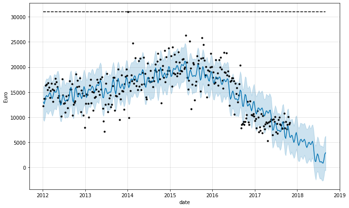
fig = m.plot(forecast, ylabel='Euro', xlabel='date')
INFO:fbprophet:Disabling weekly seasonality. Run prophet with weekly_seasonality=True to override this.
INFO:fbprophet:Disabling daily seasonality. Run prophet with daily_seasonality=True to override this.
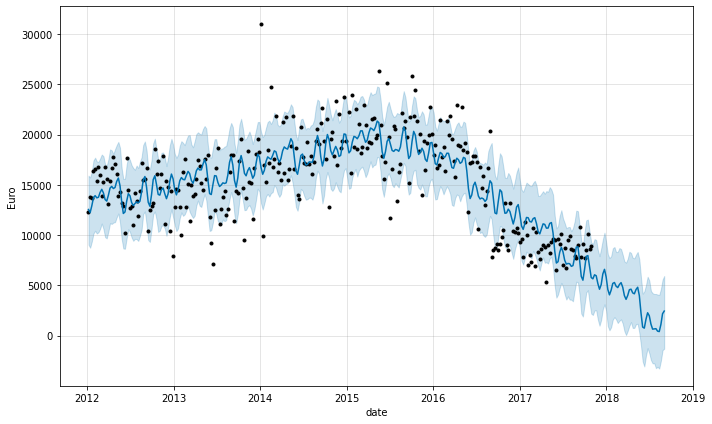
There is a decreasing trend in total alcohol sales for the store. To implement the solution, a model with logistic regression was used, where the lower value of saturation is 0 and the upper one is the maximum historical value.
del m, future
df_store_selected= df_store_sales.loc[df_store_sales['store_id'] == 0]
df_prophet=df_store_selected[['period', 'Total']]
df_prophet = df_prophet.rename(columns={'period': 'ds',
'Total': 'y'})
df_prophet['cap'] = df_prophet.y.max()
df_prophet['floor'] = 0
m = fbprophet.Prophet(growth='logistic', weekly_seasonality=True)
m.fit(df_prophet)
future = m.make_future_dataframe(44, freq='W') #MS
future['cap'] = df_prophet.y.max()
future['floor'] = 0
forecast = m.predict(future)
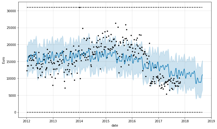
fig = m.plot(forecast, ylabel='Euro', xlabel='date')
INFO:fbprophet:Disabling daily seasonality. Run prophet with daily_seasonality=True to override this.
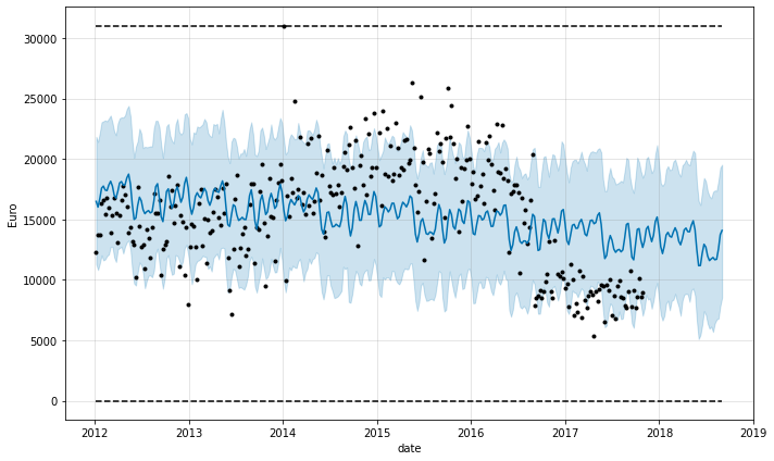
The previous model was using weekly_seasonality=True. Now check the next model by disabling it.
del m, future
df_store_selected= df_store_sales.loc[df_store_sales['store_id'] == 0]
df_prophet=df_store_selected[['period', 'Total']]

df_prophet = df_prophet.rename(columns={'period': 'ds',
                                        'Total': 'y'})
df_prophet['cap'] = df_prophet.y.max()
df_prophet['floor'] = 0

m = fbprophet.Prophet(growth='logistic')
m.fit(df_prophet)

future = m.make_future_dataframe(44, freq='W') #MS
future['cap'] = df_prophet.y.max()
future['floor'] = 0

forecast = m.predict(future)
fig = m.plot(forecast, ylabel='Euro', xlabel='date')
INFO:fbprophet:Disabling weekly seasonality. Run prophet with weekly_seasonality=True to override this.
INFO:fbprophet:Disabling daily seasonality. Run prophet with daily_seasonality=True to override this.
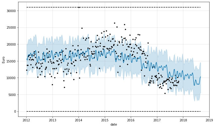
For standardization: The future dataframe should have original, not-standardized values, and the forecasted values should also not be standardized. For predictions, Prophet will apply the same standardization offset and scale used in fitting.
https://github.com/facebook/prophet/issues/484
https://github.com/facebook/prophet/issues/1392#issuecomment-602892389
Box-Cox transformation despite the information above
from scipy import stats
del m, future
df_store_selected= df_store_sales.loc[df_store_sales['store_id'] == 0]
df_prophet=df_store_selected[['period', 'Total']]
df_prophet = df_prophet.rename(columns={'period': 'ds',
'Total': 'y'})
df_prophet.y=stats.boxcox(df_prophet.y)[0]
df_prophet['cap'] = df_prophet.y.max()
df_prophet['floor'] = 0
m = fbprophet.Prophet(growth='logistic')
m.fit(df_prophet)
future = m.make_future_dataframe(44, freq='W') #MS
future['cap'] = df_prophet.y.max()
future['floor'] = 0
forecast = m.predict(future)
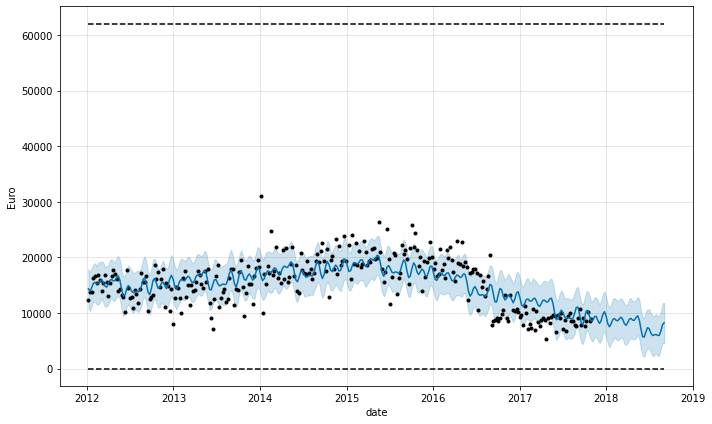
fig = m.plot(forecast, ylabel='Euro', xlabel='date')
INFO:fbprophet:Disabling weekly seasonality. Run prophet with weekly_seasonality=True to override this.
INFO:fbprophet:Disabling daily seasonality. Run prophet with daily_seasonality=True to override this.
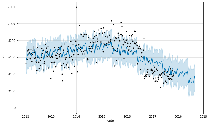
Lambda
df_store_selected= df_store_sales.loc[df_store_sales['store_id'] == 0]
df_prophet=df_store_selected[['period', 'Total']]

df_prophet['floor'] = 0
df_prophet = df_prophet.rename(columns={'period': 'ds',
                                        'Total': 'y'})

stats.boxcox(df_prophet.y)[1]
0.8974534720944913
Using the Box-Cox transformation, the data is more within the upper and thelower yhat range. However, that in making the reverse transformation, the yhat ranges will be wider than in the previous model.
https://facebook.github.io/prophet/docs/seasonality,_holiday_effects,_and_regressors.html#additional-regressors
“The extra regressor must be known for both the history and for future dates. It thus must either be something that has known future values (such as nfl_sunday), or something that has separately been forecasted elsewhere. Prophet will also raise an error if the regressor is constant throughout the history, since there is nothing to fit from it.
Extra regressors are put in the linear component of the model, so the underlying model is that the time series depends on the extra regressor as either an additive or multiplicative factor (see the next section for multiplicativity).”
When using additional regressors, it is possible to predict the data (y as search value = Total) based on each type of alcohol.
In the final version, it was decided to select several types of alcohols to check the fit of the model.
Final version
Prophet model
By selecting the chosen store, make sure that the available data will allow sufficient analysis of sales over a certain period (see store_sales_per_category section -> Usability of the data).
Choose id of the store
store_id_chosen = 0
from fbprophet.diagnostics import performance_metrics, cross_validation
Model based on all date points
def prophet_predict(store_id_chosen: int,
                    df_store_sales: pd.DataFrame,
                    multiplier: int,
                    growth_fbprophet: str,
                    *column_types):

  df_store_sales= df_store_sales.loc[df_store_sales['store_id'] == store_id_chosen]
  df_prophet=df_store_sales[np.asarray(column_types)]

  m_full = fbprophet.Prophet(growth=growth_fbprophet)
  df_forecast_regressors = pd.DataFrame([], columns=['ds'])

  #predict additional regressors
  for element in column_types[2:]:

    m=fbprophet.Prophet(growth=growth_fbprophet)
    df_inside = df_prophet.rename(columns={'period': 'ds',
                                           element: 'y'})
    df_inside['floor'] = 0
    df_inside['cap'] = df_inside.y.max()
    m.fit(df_inside[['ds', 'y', 'floor', 'cap']])

    future = m.make_future_dataframe(44, freq='W') #MS  52
    future['cap'] = df_inside.y.max()
    future['floor'] = 0
    forecast = m.predict(future)

    #merge values into df
    df_forecast_regressors = df_forecast_regressors.merge(forecast[['ds', 'yhat']],
                                                          on='ds',
                                                          how='outer')

    df_forecast_regressors = df_forecast_regressors.rename(columns={'yhat': element})
    #add regressor layer into full model
    m_full.add_regressor(element)

  df_prophet = df_prophet.rename(columns={'period': 'ds',
                                          'Total': 'y'})
  df_prophet['cap'] = multiplier*df_prophet.y.max()
  df_prophet['floor'] = 0

  m_full.fit(df_prophet)

  future_full = m_full.make_future_dataframe(44, freq='W') #MS  52
  future_full['cap'] = multiplier*df_prophet.y.max()
  future_full['floor'] = 0

  array_types=np.asarray(column_types[2:])
  array_types=np.append(array_types, 'ds')
  future_full = future_full.merge(df_forecast_regressors[array_types],
                                  on='ds',
                                  how='left')

  forecast_full = m_full.predict(future_full)
  fig = m_full.plot(forecast_full,
                    ylabel='Euro',
                    xlabel='date')

  #cutoff should be adjusted manually!
  #more information about cross validation https://facebook.github.io/prophet/docs/diagnostics.html
  df_cv = cross_validation(m_full,
                           initial='1800 days',
                           period='180 days',
                           horizon = '270 days')
  df_p = performance_metrics(df_cv)

  return forecast_full, fig, df_p, df_cv
In the next section of the code, please specify the chosen parameters:
1 - multiplier for logistic forecast (use e.g. 2 to change twice the cap value in the model, but use only 1 for linear approach).
‘linear’/’logistic’ - choose the model specification
‘period’, ‘Total’, ‘Gin’- the first two elements are required, additional regressors as Gin, Whiskey etc. are optionally
forecast_second_approach, fig_second_approach, df_p_metrics, df_cv = (
    prophet_predict(store_id_chosen,
                    df_store_sales,
                    1,
                    'linear',
                    'period',
                    'Total',
                    'Gin'))
INFO:fbprophet:Disabling weekly seasonality. Run prophet with weekly_seasonality=True to override this.
INFO:fbprophet:Disabling daily seasonality. Run prophet with daily_seasonality=True to override this.
INFO:fbprophet:Disabling weekly seasonality. Run prophet with weekly_seasonality=True to override this.
INFO:fbprophet:Disabling daily seasonality. Run prophet with daily_seasonality=True to override this.
INFO:fbprophet:Making 1 forecasts with cutoffs between 2017-02-01 00:00:00 and 2017-02-01 00:00:00


HBox(children=(FloatProgress(value=0.0, max=1.0), HTML(value='')))
Logistic version
forecast_second_approach, fig_second_approach, df_p_metrics, df_cv = (
    prophet_predict(store_id_chosen,
                    df_store_sales,
                    1,
                    'logistic',
                    'period',
                    'Total',
                    'Gin'))
INFO:fbprophet:Disabling weekly seasonality. Run prophet with weekly_seasonality=True to override this.
INFO:fbprophet:Disabling daily seasonality. Run prophet with daily_seasonality=True to override this.
INFO:fbprophet:Disabling weekly seasonality. Run prophet with weekly_seasonality=True to override this.
INFO:fbprophet:Disabling daily seasonality. Run prophet with daily_seasonality=True to override this.
INFO:fbprophet:Making 1 forecasts with cutoffs between 2017-02-01 00:00:00 and 2017-02-01 00:00:00


HBox(children=(FloatProgress(value=0.0, max=1.0), HTML(value='')))
Logistic with multiplication for cap values
forecast_second_approach, fig_second_approach, df_p_metrics, df_cv = (
    prophet_predict(store_id_chosen,
                    df_store_sales,
                    2,
                    'logistic',
                    'period',
                    'Total',
                    'Gin'))
INFO:fbprophet:Disabling weekly seasonality. Run prophet with weekly_seasonality=True to override this.
INFO:fbprophet:Disabling daily seasonality. Run prophet with daily_seasonality=True to override this.
INFO:fbprophet:Disabling weekly seasonality. Run prophet with weekly_seasonality=True to override this.
INFO:fbprophet:Disabling daily seasonality. Run prophet with daily_seasonality=True to override this.
INFO:fbprophet:Making 1 forecasts with cutoffs between 2017-02-01 00:00:00 and 2017-02-01 00:00:00


HBox(children=(FloatProgress(value=0.0, max=1.0), HTML(value='')))
Different start date of observations
def prophet_predict_date_range(store_id_chosen: int,
df_store_sales: pd.DataFrame,
date_start_fitting: str,
multiplier: int,
growth_fbprophet: str,
*column_types):
df_store_sales= df_store_sales.loc[df_store_sales['store_id'] == store_id_chosen]
df_prophet=df_store_sales[np.asarray(column_types)]
df_prophet=df_prophet[df_prophet['period']>=date_start_fitting]
m_full = fbprophet.Prophet(growth=growth_fbprophet)
df_forecast_regressors = pd.DataFrame([], columns=['ds'])
#predict additional regressors
for element in column_types[2:]:
m=fbprophet.Prophet(growth=growth_fbprophet)
df_inside = df_prophet.rename(columns={'period': 'ds', element: 'y'})
df_inside['floor'] = 0
df_inside['cap'] = df_inside.y.max()
m.fit(df_inside[['ds', 'y', 'floor', 'cap']])
future = m.make_future_dataframe(44, freq='W') #MS 52
future['cap'] = df_inside.y.max()
future['floor'] = 0
forecast = m.predict(future)
df_forecast_regressors = df_forecast_regressors.merge(forecast[['ds', 'yhat']],
on='ds',
how='outer')
df_forecast_regressors = df_forecast_regressors.rename(columns={'yhat': element})
m_full.add_regressor(element)
df_prophet['floor'] = 0
df_prophet = df_prophet.rename(columns={'period': 'ds',
'Total': 'y'})
df_prophet['cap'] = multiplier*df_prophet.y.max()
m_full.fit(df_prophet)
future_full = m_full.make_future_dataframe(44, freq='W') #MS 52
future_full['cap'] = multiplier*df_prophet.y.max()
future_full['floor'] = 0
array_types=np.asarray(column_types[2:])
array_types=np.append(array_types, 'ds')
future_full = future_full.merge(df_forecast_regressors[array_types],
on='ds',
how='left')
forecast_full = m_full.predict(future_full)
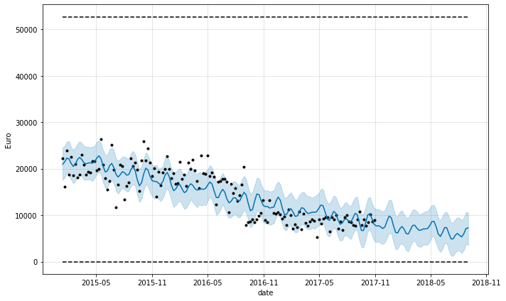
fig = m_full.plot(forecast_full, ylabel='Euro', xlabel='date')
#cutoff should be adjucted manually
df_cv = cross_validation(m_full,
initial='730 days',
period='180 days',
horizon = '270 days')
df_p = performance_metrics(df_cv)
return forecast_full, fig, df_p, df_cv
‘2015-01-01’ enter start date for forecast
forecast_second_approach, fig_second_approach, df_p_metrics, df_cv = (
    prophet_predict_date_range(
        store_id_chosen,
        df_store_sales,
        '2015-01-01',
        2,
        'logistic',
        'period',
        'Total',
        'Gin'))
INFO:fbprophet:Disabling weekly seasonality. Run prophet with weekly_seasonality=True to override this.
INFO:fbprophet:Disabling daily seasonality. Run prophet with daily_seasonality=True to override this.
INFO:fbprophet:Disabling weekly seasonality. Run prophet with weekly_seasonality=True to override this.
INFO:fbprophet:Disabling daily seasonality. Run prophet with daily_seasonality=True to override this.
INFO:fbprophet:Making 1 forecasts with cutoffs between 2017-02-01 00:00:00 and 2017-02-01 00:00:00


HBox(children=(FloatProgress(value=0.0, max=1.0), HTML(value='')))
#from fbprophet.plot import plot_cross_validation_metric
fig = fbprophet.plot.plot_cross_validation_metric(df_cv, metric='mape')
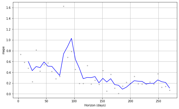
df_p_metrics.head()
| horizon | mse | rmse | mae | mape | mdape | coverage | |
|---|---|---|---|---|---|---|---|
| 0 | 18 days | 2.032174e+07 | 4507.963676 | 4455.489368 | 0.598439 | 0.585844 | 0.333333 |
| 1 | 25 days | 1.342665e+07 | 3664.239998 | 3544.375524 | 0.429956 | 0.478417 | 0.666667 |
| 2 | 32 days | 1.656929e+07 | 4070.539116 | 3849.406295 | 0.506169 | 0.478417 | 0.666667 |
| 3 | 39 days | 1.865996e+07 | 4319.718001 | 4115.942535 | 0.486830 | 0.420400 | 0.333333 |
| 4 | 46 days | 2.337920e+07 | 4835.204350 | 4800.941722 | 0.591528 | 0.539703 | 0.000000 |
df_cv.head()
| ds | yhat | yhat_lower | yhat_upper | y | cutoff | |
|---|---|---|---|---|---|---|
| 0 | 2017-02-05 | 12195.885741 | 8493.102411 | 15952.736176 | 7045.34 | 2017-02-01 |
| 1 | 2017-02-12 | 12705.813049 | 9041.965477 | 16419.567468 | 8012.02 | 2017-02-01 |
| 2 | 2017-02-19 | 10884.179313 | 7017.838101 | 14276.419510 | 7362.05 | 2017-02-01 |
| 3 | 2017-02-26 | 13131.454210 | 9539.785105 | 16624.701770 | 10714.25 | 2017-02-01 |
| 4 | 2017-03-05 | 12495.325361 | 8618.546173 | 16072.765590 | 6886.44 | 2017-02-01 |
Clustering was done previously. In this subsection we only choose stores with same cluster label.
df_clustered = df_store_gdata.loc[df_store_gdata['store_id'] == store_id_chosen]
df_clustered_by_chosen_store= df_store_gdata.loc[df_store_gdata['cluster'] == int(df_clustered.cluster)]
df_clustered_by_chosen_store.head()
| university or college | foodstores or supermarkets or gorceries | restaurant | churches | gym | stadium | store_id | cluster | |
|---|---|---|---|---|---|---|---|---|
| 26 | 5 | 7 | 20 | 20 | 20 | 3 | 0 | 135 |
| 65 | 5 | 7 | 20 | 20 | 20 | 3 | 39 | 135 |
| 66 | 5 | 7 | 20 | 20 | 20 | 3 | 40 | 135 |
| 210 | 4 | 6 | 20 | 20 | 20 | 3 | 184 | 135 |
| 301 | 4 | 6 | 20 | 20 | 20 | 3 | 275 | 135 |
Build a classifier using this “labelled” data:
from sklearn.model_selection import train_test_split
from sklearn.metrics import accuracy_score
from sklearn.neighbors import KNeighborsClassifier
np.random.seed(42)
train, test = train_test_split(df_store_gdata, test_size=0.20)

col_list_to_classify = ['university or college', 'foodstores or supermarkets or gorceries', 'restaurant', 'churches', 'gym', 'stadium']

X_train = train[col_list_to_classify]
y_train = train[['cluster']]

X_test = test[col_list_to_classify]
y_test = test[['cluster']]

knn = KNeighborsClassifier()
knn.fit(X_train, y_train)
res = knn.predict(X_test)
acc = accuracy_score(res.transpose(), y_test.values)
acc
0.896551724137931
By checking which cluster of stores belong to, it is needed to use knn.predict on the chosen model. Instead of using, again, clustering while adding one record (our client), the prediction using KNN Classifier gave us about 90% accuracy and is a quite good solution instead of creating new clusterization.
df_another_stores_by_cluster=df_store_merged.loc[df_store_merged['store_id'].isin(df_clustered_by_chosen_store.store_id)]
df_another_stores_by_cluster_by_the_store=df_another_stores_by_cluster.loc[df_store_merged['store_id']==store_id_chosen]
d_concurrency = {'store_id': store_id_chosen,
                 'Number of store in same cluster': df_another_stores_by_cluster.store_id.count(),
                 'Median of the competitor stores (within 5km radius from each store) in the same cluster': np.median(df_another_stores_by_cluster.total_no_stores_in_5_km),
                 'Number of competitor stores (within 5 km radius from each store) of chosen store': df_another_stores_by_cluster_by_the_store.total_no_stores_in_5_km}

df_concurrency = pd.DataFrame(data=d_concurrency)
df_concurrency
| store_id | Number of store in same cluster | Median of the competitor stores (within 5km radius from each store) in the same cluster | Number of competitor stores (within 5 km radius from each store) of chosen store | |
|---|---|---|---|---|
| 0 | 0 | 33 | 41.0 | 28 |
Interpretation
If the level of competition is lower than the median/average, this means that the store potentially has less risk of competition.
# pip freeze --local > "/content/gdrive/My Drive/Prophet/colab_installed.txt"
import sys
print(sys.version)
3.7.10 (default, Feb 20 2021, 21:17:23)
[GCC 7.5.0]