Table of contents
Stock price: jumping out and in of dividend stocks around ex dividend dates
The payment of dividends by a company is an attractive morsel for a shareholder. Such a company is better perceived because of its attractiveness and its willingness to share its profits with investors. But is it always profitable to own shares when dividends are paid? In this note, I will try to answer this question. For the analysis, I have chosen companies that regularly pay dividends on the Polish stock exchange.
Why are some people might leap the dividend?
Investing within brokerage accounts with some providers is possible in shares. These investment ways can be interesting to people who are familiar with trading on the stock market and are willing to make their own decisions. By setting up a diversified portfolio, we can buy shares in many companies. It reduces some of the possible consequences. If we invest outside our retirement accounts, and if we sell the shares at a profit or if we receive a dividend, we have to pay a tax of 19% on the profit. However, within retirement accounts, we do not have to pay this as such investing is tax-free, but only if we withdraw funds from such an account when we reach the appropriate retirement age. Skipping dividends makes sense in the case of companies with a high free float and a large capitalisation (as our sale will not have a large impact on the share price), when we want to deduct a previous loss and when we want to trade longer (19% tax must be paid by the end of April of the next year).
The amount we intend to invest in one company is PLN 10k (nonsignificant impact to the price of share).
Import data and make some cleaning steps
import pandas as pd
# The importing can be made in two ways. By download, the file and read by pd.read_csv,
# or read directly by pandas from the website. Awareness: when many attempts is made to
# the page, it may cause an internal error. It can be suspected of spam action.
# df = pd.read_csv("acp_d.csv")
df = pd.read_csv('https://stooq.pl/q/d/l/?s=acp&i=d&o=0001000')

def rename_df_stock_prices(df: pd.DataFrame) -> pd.DataFrame:
    """
    Change headers language to polish.

    Input:
        df pd.DataFrame
    Output:
        df pd.DataFrame
    """
    df = df.rename(columns={"Data": "Date",
                            "Otwarcie": "Opening",
                            "Najwyzszy": "Highest",
                            "Zamkniecie":"Closing",
                            "Najnizszy": "Lowest",
                            "Wolumen": "Volume"})
    df['Date'] = pd.to_datetime(df['Date'], format='%Y-%m-%d')
    return df

df = rename_df_stock_prices(df)
df
| Date | Opening | Highest | Lowest | Closing | Volume | |
|---|---|---|---|---|---|---|
| 0 | 1998-06-02 | 10.602 | 10.602 | 10.602 | 10.602 | 577707 |
| 1 | 1998-06-03 | 11.648 | 11.648 | 11.648 | 11.648 | 221464 |
| 2 | 1998-06-04 | 12.694 | 12.694 | 12.694 | 12.694 | 655891 |
| 3 | 1998-06-05 | 12.847 | 12.847 | 12.847 | 12.847 | 252087 |
| 4 | 1998-06-08 | 12.794 | 12.794 | 12.794 | 12.794 | 141804 |
| ... | ... | ... | ... | ... | ... | ... |
| 5758 | 2021-06-07 | 70.050 | 71.100 | 69.900 | 70.150 | 220481 |
| 5759 | 2021-06-08 | 70.100 | 71.300 | 69.800 | 70.900 | 84408 |
| 5760 | 2021-06-09 | 71.000 | 71.000 | 69.600 | 69.600 | 86795 |
| 5761 | 2021-06-10 | 69.650 | 71.000 | 69.650 | 70.950 | 59770 |
| 5762 | 2021-06-11 | 70.700 | 70.700 | 69.950 | 69.950 | 33492 |
5763 rows × 6 columns
Disclaimer: https://stooq.pl/pomoc/?q=9&s=acp
Modified data analysis is prone to be confused. In the case of technical analysis (AT), it is necessary to take into account supports, upward movements, or other phenomena that may determine the price movement.
# Get the information of dividend payments
import requests
from bs4 import BeautifulSoup

page = requests.get("https://stooq.pl/q/m/?s=acp")

def parse_request(page) -> pd.DataFrame:
    """
    Parse request into pd.DataFrame

    Input:
        request
    Output:
        df_list: pd.DataFrame
    """
    soup = BeautifulSoup(page.content, 'html.parser')
    df_list = pd.read_html(page.text)
    return df_list

df_list = parse_request(page)
df_list[0]
| Data | Zdarzenie | Nominalnie | Dzielnik | |
|---|---|---|---|---|
| 0 | NaN | NaN | NaN | NaN |
| 1 | NaN | UlubioneGPW, WIG20, AkcjeIndeksy, Azja, Europa... | NaN | NaN |
| 2 | NaN | NaN | NaN | NaN |
| 3 | NaN | Market On-line | NaN | NaN |
| 4 | NaN | NaN | NaN | NaN |
| 5 | Åro, 2 cze 2021 | Dywidenda 4.23% | 3.10000 | 1.044223 |
| 6 | czw, 4 cze 2020 | Dywidenda 4.11% | 2.87300 | 1.042857 |
| 7 | piÄ , 17 maj 2019 | Dywidenda 5.96% | 2.81910 | 1.063325 |
| 8 | piÄ , 18 maj 2018 | Dywidenda 6.68% | 2.59080 | 1.071565 |
| 9 | pon, 15 maj 2017 | Dywidenda 5.43% | 2.42580 | 1.057454 |
| 10 | piÄ , 13 maj 2016 | Dywidenda 5.41% | 2.29410 | 1.057235 |
| 11 | czw, 14 maj 2015 | Dywidenda 4.85% | 2.09060 | 1.050922 |
| 12 | pon, 19 maj 2014 | Dywidenda 5.89% | 1.78350 | 1.062545 |
| 13 | czw, 16 maj 2013 | Dywidenda 5.06% | 1.55590 | 1.053330 |
| 14 | wto, 15 maj 2012 | Dywidenda 4.64% | 1.34210 | 1.048656 |
| 15 | piÄ , 13 maj 2011 | Dywidenda 3.48% | 1.05210 | 1.036108 |
| 16 | czw, 14 paź 2010 | Prawo Poboru 0.20% | 0.05636 | 1.001957 |
| 17 | Åro, 23 cze 2010 | Dywidenda 2.54% | 0.81640 | 1.026103 |
| 18 | pon, 8 cze 2009 | Dywidenda 1.83% | 0.57610 | 1.018601 |
| 19 | czw, 19 cze 2008 | Dywidenda 0.95% | 0.29633 | 1.009549 |
| 20 | Åro, 13 cze 2007 | Dywidenda 0.46% | 0.21350 | 1.004619 |
| 21 | Åro, 28 cze 2006 | Dywidenda 1.67% | 0.31865 | 1.016949 |
| 22 | NaN | NaN | NaN | NaN |
| 23 | NaN | document.write(Modernizr.svg?'<svg xmlns="http... | NaN | NaN |
# Process into pandas and convert into format='%d-%m-%Y'
df_list = pd.read_html(page.text, encoding='utf-8')

def clean_df_stock(df_list: pd.DataFrame) -> pd.DataFrame:
    """
    Cleaning df: extract date aby the regex and convert into format='%d-%m-%Y'.
    Additionally, change headers' language to English.

    Input:
        df_list pd.DataFrame
    Output:
        cleaned_df: pd.DataFrame

    """
    # Remove rows with NaNs
    cleaned_df = df_list[0].copy().dropna(thresh=2)
    cleaned_df = cleaned_df.rename(columns={"Data": "Date",
                                            "Zdarzenie": "Event",
                                            "Nominalnie": "Nominal",
                                            "Dzielnik": "Divider"})
    date_dict = {
    "sty": "01",
    "lut": "02",
    "mar":"03",
    "kwi": "04",
    "maj":"05",
    "cze":"06",
    "lip":"07",
    "sie":"08",
    "wrz":"09",
    "paź":"10",
    "lis":"11",
    "gru":"12"}

    # Extract date from the Data column
    cleaned_df.loc[:,'Date'] = cleaned_df.loc[:,'Date'].str.extract('(\d+\s\w+\s\d+)', expand=False).str.strip()
    cleaned_df.loc[:,'Date'] = cleaned_df.loc[:,'Date'].replace(date_dict, regex=True)
    cleaned_df.loc[:,'Date'] = cleaned_df.loc[:,'Date'].replace(' ', '-', regex=True)
    cleaned_df.loc[:,'Date'] = pd.to_datetime(cleaned_df.loc[:,'Date'], format='%d-%m-%Y')

    return cleaned_df

cleaned_df = clean_df_stock(df_list)
cleaned_df
| Date | Event | Nominal | Divider | |
|---|---|---|---|---|
| 5 | 2021-06-02 | Dywidenda 4.23% | 3.10000 | 1.044223 |
| 6 | 2020-06-04 | Dywidenda 4.11% | 2.87300 | 1.042857 |
| 7 | 2019-05-17 | Dywidenda 5.96% | 2.81910 | 1.063325 |
| 8 | 2018-05-18 | Dywidenda 6.68% | 2.59080 | 1.071565 |
| 9 | 2017-05-15 | Dywidenda 5.43% | 2.42580 | 1.057454 |
| 10 | 2016-05-13 | Dywidenda 5.41% | 2.29410 | 1.057235 |
| 11 | 2015-05-14 | Dywidenda 4.85% | 2.09060 | 1.050922 |
| 12 | 2014-05-19 | Dywidenda 5.89% | 1.78350 | 1.062545 |
| 13 | 2013-05-16 | Dywidenda 5.06% | 1.55590 | 1.053330 |
| 14 | 2012-05-15 | Dywidenda 4.64% | 1.34210 | 1.048656 |
| 15 | 2011-05-13 | Dywidenda 3.48% | 1.05210 | 1.036108 |
| 16 | 2010-10-14 | Prawo Poboru 0.20% | 0.05636 | 1.001957 |
| 17 | 2010-06-23 | Dywidenda 2.54% | 0.81640 | 1.026103 |
| 18 | 2009-06-08 | Dywidenda 1.83% | 0.57610 | 1.018601 |
| 19 | 2008-06-19 | Dywidenda 0.95% | 0.29633 | 1.009549 |
| 20 | 2007-06-13 | Dywidenda 0.46% | 0.21350 | 1.004619 |
| 21 | 2006-06-28 | Dywidenda 1.67% | 0.31865 | 1.016949 |
def get_only_dividend_event(cleaned_df: pd.DataFrame) -> pd.DataFrame:
    """
    Get only divident (pl: Dywidenda) event from dataframe

    Input:
        cleaned_df pd.DataFrame
    Return:
        cleaned_df pd.DataFrame

    """
    cleaned_df[cleaned_df['Event'].str.contains("Dywidenda")]
    return cleaned_df

cleaned_df = get_only_dividend_event(cleaned_df)
Calculate potential profit of dividend leaping
Get the highest profit
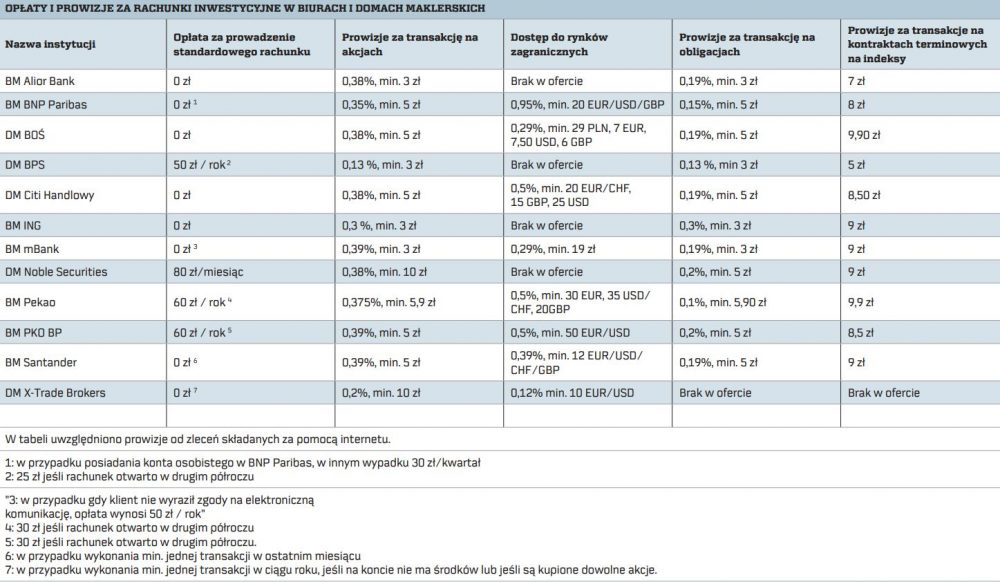
Assuming that the average provision for buy/sell share is equal to 0.38%, the calculation has been made. The maximum of ‘Highest’ column price value (before the dividend) has been taken into account and the ‘Lowest’ price (after the dividend payment).
F = highestmax - lowestmin - provision * (highestmax + lowestmin) - dividend

Source: https://pieniadze.rp.pl/wp-content/uploads/2020/02/biura_maklerskie_oplaty_prowizje.jpg
import numpy as np
import matplotlib.pyplot as plt

from datetime import date
from sklearn.preprocessing import MinMaxScaler

# Set setting for plot of the transform stock price
%matplotlib inline
plt.rcParams['figure.figsize'] = [15, 10]
plt.style.use('seaborn-whitegrid')
fig = plt.figure()
ax = plt.axes()

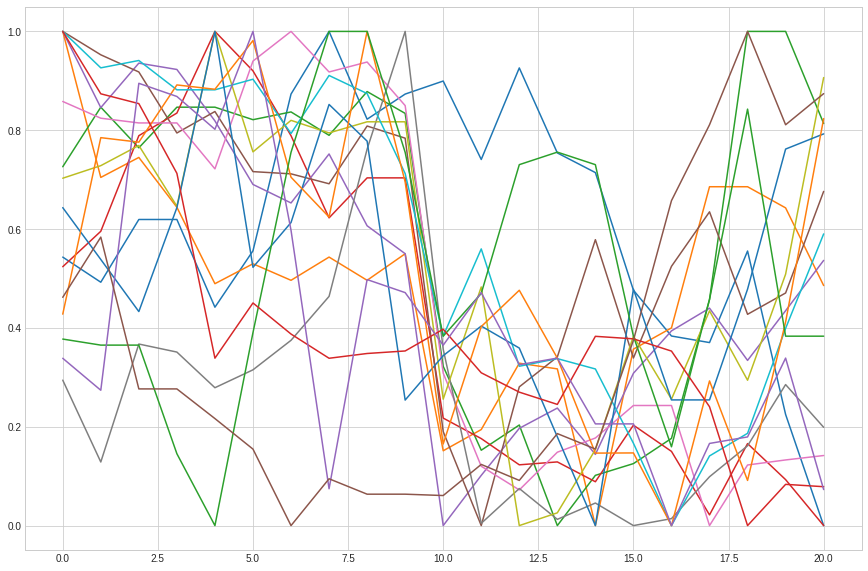
# Create numpy range for 10 days before dividend, dividend day, and 10 days after
x = np.arange(0, 21, 1)
k=0

list_of_profits = []
list_of_minmaxscaled = []
list_of_scaled = []
list_of_noscaled = []

pd.options.mode.chained_assignment = None

for index, row in cleaned_df.iterrows():
    try:
        dividend_day = pd.to_datetime(row['Date'], format='%Y-%m-%d')
        idx = df[df.Date == dividend_day].index

        # Get the stock prices 10 session before dividend and 10 after
        filtered_idx = (idx - 10).union(idx+10)
        filtered_idx = filtered_idx[filtered_idx > 0]
        df_index_range = df.iloc[filtered_idx].reset_index()

        # Based on filtering condition get only data between the range
        df_range_date = df.loc[(df["Date"] >= df_index_range['Date'][0]) &
                        (df['Date'] <= df_index_range['Date'][1])]

        list_of_noscaled.append(df_range_date.copy())

        list_of_scaled.append(df_range_date)
        list_of_scaled[k].loc[df_range_date.Date<str(dividend_day),
                              ['Opening', 'Highest', 'Lowest', 'Closing']] += float(row['Nominal'])

        maximum = list_of_scaled[k].loc[list_of_scaled[k].Date<str(dividend_day), ['Highest']].max()
        minimum = list_of_scaled[k].loc[list_of_scaled[k].Date>=str(dividend_day), ['Lowest']].min()

        profit = (maximum.values-minimum.values)-maximum.values*0.0038-minimum.values*0.0038-float(row['Nominal'])
        list_of_profits.append(profit)

        # Use MinMaxScaler for better visual changes in the stock prices
        scaler = MinMaxScaler()
        df_range_date = scaler.fit_transform(df_range_date[['Closing']]).T
        list_of_minmaxscaled.append(df_range_date)

        plt.plot(x, df_range_date.ravel())

        k+=1

    except IndexError:
        print("Insufficient data information. Probably the dataset doesn't have ten days after payment dividend")

plt.show()
Insufficient data information. Probably the dataset doesn't have ten days after payment dividend

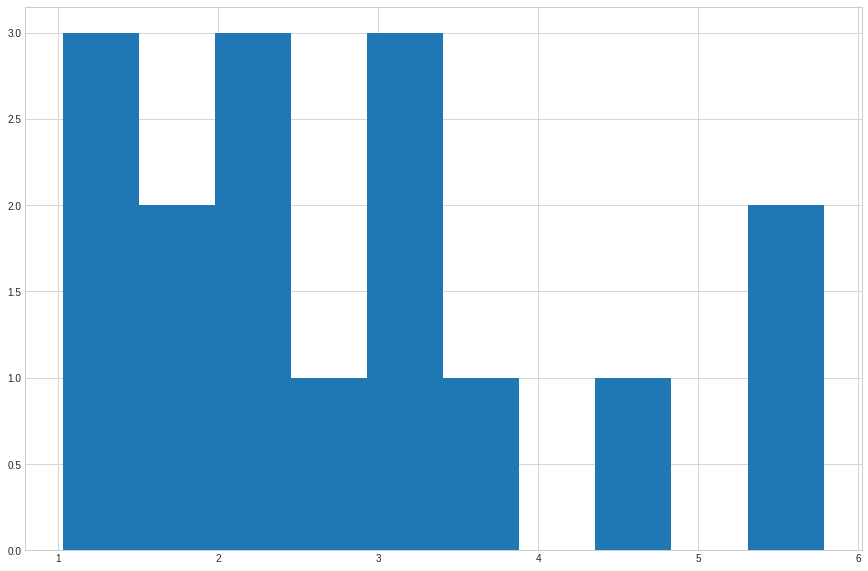
counts, bins = np.histogram(list_of_profits)
plt.hist(bins[:-1], bins, weights=counts)
(array([3., 2., 3., 1., 3., 1., 0., 1., 0., 2.]),
 array([1.02662962, 1.50259882, 1.97856802, 2.45453721, 2.93050641,
        3.40647561, 3.88244481, 4.35841401, 4.8343832 , 5.3103524 ,
        5.7863216 ]),
 <a list of 10 Patch objects>)

adjusted approach
Life has proved to be not perfect. For chosen company, we got more profit than holding the shares for dividend (#toTheMoon). Some of you might be long-term investors (by choice or by having a large loss on your shares, so you don’t sell - high five). For adding a more adjusted price of selling and buying, let’s get mean from the highest and lowest share’s price per day.
def calculate_adjusted_profit(cleaned_df: pd.DataFrame, df: pd.DataFrame) -> list:
    """
    Calculate adjusted profit:
    mean from the highest and lowest share's price per day

    Input:
        cleaned_df: pd.DataFrame
        df: pd.DataFrame
    Output:
        list_of_profits: list

    """
    # Create numpy range for 10 days before dividend, dividend day, and 10 days after
    x = np.arange(0, 21, 1)
    k=0

    list_of_profits = []
    list_of_minmaxscaled = []
    list_of_scaled = []
    list_of_noscaled = []

    for index, row in cleaned_df.iterrows():
        try:
            dividend_day = pd.to_datetime(row['Date'], format='%Y-%m-%d')
            idx = df[df.Date == dividend_day].index

            # Get the stock prices 10 session before dividend and 10 after
            filtered_idx = (idx - 10).union(idx+10)
            filtered_idx = filtered_idx[filtered_idx > 0]
            df_index_range = df.iloc[filtered_idx].reset_index()

            # Based on filtering condition get only data between the range
            df_range_date = df.loc[(df["Date"] >= df_index_range['Date'][0]) &
                            (df['Date'] <= df_index_range['Date'][1])]

            list_of_noscaled.append(df_range_date.copy())

            list_of_scaled.append(df_range_date)
            list_of_scaled[k].loc[df_range_date.Date<str(dividend_day),
                                  ['Opening', 'Highest', 'Lowest', 'Closing']] += float(row['Nominal'])

            maximum = list_of_scaled[k].loc[list_of_scaled[k].Date<str(dividend_day), ['Highest', 'Lowest']]
            maximum = ((maximum.Highest+maximum.Lowest)/2).max()

            minimum = list_of_scaled[k].loc[list_of_scaled[k].Date>=str(dividend_day), ['Highest', 'Lowest']]
            minimum = ((minimum.Highest+minimum.Lowest)/2).min()

            profit = (maximum-minimum)-maximum*0.0038-minimum*0.0038-float(row['Nominal'])
            list_of_profits.append(profit)

            # Use MinMaxScaler for better visual changes in the stock prices
            scaler = MinMaxScaler()
            df_range_date = scaler.fit_transform(df_range_date[['Closing']]).T
            list_of_minmaxscaled.append(df_range_date)

            plt.plot(x, df_range_date.ravel())

            k+=1

        except IndexError:
            print("Insufficient data information. Probably the dataset doesn't have ten days after payment dividend")
        except KeyError:
            print("Missing data")
            # it occurs in ASE company, where the file doesn't contain all data

    return list_of_profits

list_of_profits = calculate_adjusted_profit(cleaned_df, df)
Insufficient data information. Probably the dataset doesn't have ten days after payment dividend

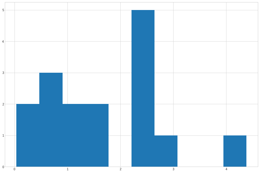
counts, bins = np.histogram(list_of_profits)
plt.hist(bins[:-1], bins, weights=counts)
(array([2., 3., 2., 2., 0., 5., 1., 0., 0., 1.]),
 array([0.03746272, 0.47188621, 0.90630971, 1.3407332 , 1.77515669,
        2.20958018, 2.64400368, 3.07842717, 3.51285066, 3.94727415,
        4.38169765]),
 <a list of 10 Patch objects>)

Based on a “adjusted” scenario, it can be concluded that for Asseco Poland, skipping a dividend in a short period before it is paid may give us a higher return than holding for a longer period.
By comparing companies that regularly pay dividends, those listed in the table were selected. They are notable for having paid dividends year on year regardless of the coronavirus pandemic.
| Company | Ticker | For how many years has the dividend been paid continuously | Dividend rate | Sector |
|---|---|---|---|---|
| SNIEZKA | SKA | 17 | 2,9% | Chemistry |
| NEUCA | NEU | 16 | 1,9% | Pharmaceutical |
| DOMDEV | DOM | 14 | 9,3% | Construction |
| WAWEL | WWL | 13 | 5,5% | Foods |
| UNIBEP | UNI | 12 | 3,0% | Construction |
| ASSECOBS | ABS | 12 | 5,1% | Informatics |
| ASSECOSEE | ASE | 11 | 1,6% | Informatics |
| KETY | KTY | 11 | 7,4% | Metallurgical |
| AMBRA | AMB | 11 | 4,0% | Foods |
Source (PL): https://strefainwestorow.pl/artykuly/dywidendy/20200914/9-najlepszych-dywidendowych-spolek
stock_list_company=['ska', 'neu', 'dom', 'wwl', 'uni', 'abs', 'ase', 'amb']
data_profit = pd.DataFrame()

for company in stock_list_company:
    df = pd.read_csv('https://stooq.pl/q/d/l/?s='+company+'&i=d&o=0001000')
    df = rename_df_stock_prices(df)

    page = requests.get("https://stooq.pl/q/m/?s="+company)
    df_list = parse_request(page)

    cleaned_df = clean_df_stock(df_list)
    cleaned_df = get_only_dividend_event(cleaned_df)
    profits = calculate_adjusted_profit(cleaned_df, df)

    data_profit = data_profit.append([profits.copy()])

data_profit = data_profit.transpose()
data_profit.columns = stock_list_company
data_profit = data_profit.round(2)
data_profit.describe()
Missing data


<bound method NDFrame.describe of      ska    neu    dom     wwl   uni   abs   ase   amb
0  -1.16   1.41  13.86   11.24  0.64 -0.17 -0.18  0.89
1  -0.02  10.59   0.73   12.17  0.20  1.51  0.11 -0.00
2   1.40  -0.33   4.86  -23.69  0.25  3.02  1.29  0.54
3   0.63  10.87  -0.85   28.32  1.44  1.45  0.40  0.46
4  -1.01  17.52   1.87  -10.15  1.12  0.94  0.17  0.11
5   1.56   4.24   0.76   28.86  1.10  1.10  0.18  0.06
6   2.84  -2.92   1.17   42.30 -0.01  0.53  0.43  0.32
7   3.11  22.63   0.68  137.60  0.28 -0.28  0.17 -0.19
8   2.32   3.46   0.06   -5.86  0.40  0.35  0.50 -0.08
9  -0.20  -1.03  -0.42   14.99 -0.10  0.70  0.63  0.24
10  1.16  -1.06   2.24    7.47  0.22  0.68   NaN  0.39
11  0.81  -1.16   2.62   15.29  0.10  0.26   NaN  0.28
12  3.66   3.60   4.48   -9.90   NaN   NaN   NaN  1.93
13  1.18   7.96   5.32    5.73   NaN   NaN   NaN  0.22
14  0.72   2.42    NaN     NaN   NaN   NaN   NaN  0.01>
Conclusions
Based on the 50% percentyle, for all selected company, we have more profit if we skip the dividend. It is hard to say on which should we sell owned shares and buy again them. If it were that simple to pick the best days in regards to profits, we’d be millionaires.
For me, this project gave me opportunities to processing data by the pandas library. I also get some web scrapping techniques. As the project developed, I tried to apply new solutions to make the project more realistic and simulate real situations like commissions or taking the average min/max rate of a given day to eliminate excessive fluctuations.